Modeling a realistic dynamical model for high energy heavy ion collisions Open Access

Abstract

1. Introduction

Since the Relativistic Heavy Ion Collider (RHIC) at Brookhaven National Laboratory (BNL) started operating in 2000, a lot of discoveries have been made and a lot of insight related to quantum chromodynamics (QCD) phase transition and the quark–gluon plasma (QGP) has been gained. One of the most physically interesting and surprising outcomes at RHIC is the production of the strongly interacting QGP (sQGP). This accomplishment was realized by combining investigations from both experimental [1] and theoretical [2] sides. Because the QGP had been believed to be a weakly interacting system like the ideal gas, the discovery of sQGP opened up a new paradigm for the understanding of high temperature and/or high density QCD.

The highlights of the RHIC experiments were (i) strong elliptic flow, which suggests early thermalization and early formation of collectivity; (ii) strong jet quenching, which confirms the formation of hot and dense matter in collisions; (iii) constituent quark number scaling of the elliptic flow, which indicates the formation of deconfined hot quark soup [3]. From studies of these experimental results with relativistic hydrodynamical models, the jet energy loss mechanism, and recombination models, the discovery of sQGP at RHIC [4] was accomplished. Furthermore, heavy ion collision operation at the Large Hadron Collider (LHC), the collision energy of which is around 15 times as large as that at RHIC, started in 2010. Such a high energy collision experiment gives us an opportunity to perform further investigations on the QCD diagram.

Figure 1 shows a schematic sketch of the time evolution in relativistic heavy ion collisions on the basis of present understanding. When two heavy ions are accelerated to high energy, an extreme state that is described by static color charge and classical gluon fields, called the color glass condensate (CGC) state, is realized inside each heavy ion. At the collision of the two heavy ions, high energy prompt photons, Drell–Yan dileptons, and jets are produced by hard scattering of quarks and gluons. After the collision thermalization is achieved in a short time. During that time, prethermal photons and dileptons are created and the entropy of the fireball increases. If the collision energy is large enough, QGP is also produced at this stage. Then hydrodynamical expansion starts, and a lot of interesting physical processes occur: collective flow formation, jet quenching, production of thermal photons and dileptons, and so on. As the temperature and density of the fireball decreases, hadronization of the QGP phase takes place. To understand the hadronization mechanism in relativistic heavy ion collisions, the recombination/coalescence mechanism and the fragmentation mechanism are employed. Gradually the mean free path between hadrons becomes large, and eventually freezeout happens. At this stage, final state interactions play an important role.

Fig. 1.

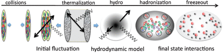
Schematic sketch of relativistic heavy ion collisions. The wavy lines stand for photons and the arrows stand for jets.

Open in new tabDownload slide

The present understanding of heavy ion collisions strongly suggests (Fig. 1) that multi-module modeling is indispensable for the description of the entire history of heavy ion collisions. Knowledge of the dominant physics at each stage has been accumulated, but a comprehensive model is still missing. For the construction of such a multi-module model, hydrodynamical models are a promising starting point, because at present these are considered one of the most reliable and successful dynamical models for comprehensively understanding experimental data at RHIC and LHC, especially for the description of the QGP phase. At the same time, it is easy to implement the latest developments in the physics of heavy ion collisions, such as fluctuating initial conditions, the lattice QCD-inspired equation of state, the recombination mechanism for hadronization, and final state interactions in freezeout processes, into a hydrodynamical model, as we will describe later in detail.

In Tables 1 and 2 current hydrodynamical models are listed. In line with the physical picture shown in Fig. 1, in particular, we pick up and compare the following features of each hydrodynamical model: the dimension of hydrodynamical expansion (dim), initial condition (IC), equation of state (EoS), and treatment of freezeout process. In addition, we also compare the numerical schemes in solving the relativistic hydrodynamical equation and observables calculated in each model in the tables. The importance of utilizing proper numerical schemes in solving the relativistic hydrodynamical equation will be discussed in Sect. 4. The recent developments in relativistic viscous hydrodynamical models are remarkable. From the point of view of multi-module modeling, however, the status of ideal hydrodynamical models is considered to be more mature.

In this article, we outline the modeling of a realistic dynamical model for the description of relativistic heavy ion collisions in line with the physical picture shown by the schematic sketch (Fig. 1). In the discussion, we refer to and compare with experimental data from SPS, RHIC, and LHC. The article is organized as follows. In Sect. 2, we review the initial conditions for hydrodynamical models from the conventional Glauber type one to the latest attempt to include event-by-event fluctuating initial conditions. In Sect. 3, we present the basic concepts and ingredients of both ideal and viscous hydrodynamics such as the relativistic hydrodynamical equation, equations of state, and transport coefficients. We will also discuss interplay between jets, the medium, and hydrodynamical expansion. In Sect. 4, we review the numerical schemes that are listed in Tables 1 and 2 and show the result of a newly developed scheme by one of the authors and her collaborators for a relativistic viscous hydrodynamical model. In Sect. 5, we explain the recombination model and show its utility in understanding hadron observables and the QCD phase diagram. In Sect. 6, we explain chemical and thermal freezeout processes and discuss the effects of final state interactions by comparing theoretical calculations and experimental data. Section 7 is devoted to the summary and conclusions.

2. Initial conditions

The hydrodynamical equations of motion require inputs of initial conditions for all their dynamical variables, which are then evolved forward in time. These initial conditions are outside of the framework of hydrodynamical models and have to be determined by other means. Physically, they are determined by the process during the initial collision of the nuclei and the succeeding stage that makes the system approach equilibrium, which is eventually reached at a time τ₀. Note that τ₀, in principle, can depend on the coordinate space rapidity η, while in practice it is assumed to be independent of η. The equilibration time is a parameter since the equilibration mechanisms are still under debate and first principle determination of the initial conditions of the equilibrated plasma phase has not been achieved. [20,21].

Historically, parameterized initial conditions for entropy density (or alternatively the energy densities) and the net baryon density have been used [7,22–24]. In the transverse plane these distributions have been mainly parameterized based on Glauber type models of nuclear collisions. In the longitudinal direction initial distributions inspired by Bjorken's scaling solution are often used. Then a few parameters remain to be fixed additionally in the initial condition, such as the maximum values of the energy or entropy density, and net baryon density. They are usually fixed by comparison with experimental data on single particle rapidity distributions and transverse momentum spectra.

As a first trial, one can choose to set the initial longitudinal flow to Bjorken's scaling solution [25], and one can set the initial transverse flow to zero. This simplest initial flow profile has served as the basis for all further investigation. The possibility of the existence of an initial transverse flow at τ₀ was discussed, e.g., by Kolb and Rapp [26]. The initial flow improves the results for P_T spectra and reduces the anisotropy.

This suggests that HBT analyses may be a sensitive tool for the determination of the initial longitudinal flow. We note that, for the analysis of the final state longitudinal flow, Yano–Koonin parameterization is effective. Hydrodynamical calculations during the early RHIC years did show serious disagreement with experimental data, especially for the ratio of R_out/R_side, leading to the notion of the HBT puzzle [27]. It turned out that the solution of the HBT puzzle is not so simple because it is related to all stages of the hydrodynamical model: initial conditions, the equation of state, viscosity effect, and final state interactions. Pratt [28] showed that this HBT puzzle comes not from a single shortcoming of hydrodynamical models, but from the combination of several effects; it is solved by mainly prethermal acceleration, a stiffer equation of state, and the viscosity effect.

Let us come back to the apparent early thermalization times found at RHIC. Usually it is argued that small initial times τ₀ are needed to describe the elliptic flow data as the elliptic flow builds up at the earliest stage of expansion when the eccentricity of the fireball is largest [29,30]. However, we note that, with suitable sets of initial conditions and freezeout temperatures, a larger initial proper time is, in fact, also compatible with the data. Luzum and Romatschke show that three very different sets of initial and freezeout temperatures (T_i, T_f)—(0.29,0.14) GeV with τ₀=2 fm, (0.36,0.15) GeV with τ₀=1 fm, and (0.43,0.16) GeV with τ₀=0.5 fm—provide almost identical differential elliptic flows in their viscous hydrodynamical calculation [14]. This suggests that better constraints on initial conditions are indispensable to avoid incorrect conclusions from comparisons of hydrodynamical calculations with experimental data.

Other approaches have been also taken in generating initial conditions. Color glass condensate-inspired initial conditions are becoming increasingly popular (Tables 1 and 2). They feature larger eccentricities of the initial energy profile than Glauber-based models, which has significant implications for elliptic flow [31]. In these models, additional dissipation during the early quark–gluon plasma stage is needed in order to achieve agreement with experiments [4,31]. Others models include the string rope model [32] and the pQCD + saturation model [33]. In the latter, the initial time τ₀ is given by the inverse of the saturation scale, which is very small, i.e., τ=0.18 (0.10) fm at RHIC (LHC).

More recently there has been a push to implement the effects of event-by-event fluctuations in the initial conditions. In the NEXSPHERIO hydro model, each event is created by the event generator NeXus [3]. First they found that the existence of fluctuation in initial conditions improves the behavior of the elliptic flow as a function of the rapidity in hydrodynamical calculations [34]. They showed that the two artificial bumps in the elliptic flow as a function of the rapidity [23] disappear if they take into account initial fluctuations.

An interesting observable, a “Mach-cone-like structure”, which is an angular correlation with the leading jet particle, was reported at RHIC [35,36]. At first the origin of the structure is considered as the remnant of the interactions between the jets and the medium ([18]–[26] in Ref. [35]). Models succeeded in giving a qualitative interpretation of the structure, but they were not so successful in quantitatively describing the experimental data. For the first time, in Ref. [37] event-by-event fluctuations in the initial state were considered as a possible origin of the structure. A breakthrough of clear understanding of the Mach-cone-like structure was done by detailed experimental analyses of triangular flow and higher harmonics. Current understanding is that the Mach-cone-like structure is dominated by the triangular flow (see, e.g., Ref. [38]). The triangular flow and higher harmonics are the coefficients in the Fourier expansion of particle yields as a function of the azimuthal angle ϕ,

\begin{align}\label{eq2.1} \frac{dN}{dyd\phi} &\propto 1 + 2 v_1 \cos (\phi-\Theta_1) + 2 v_2 \cos 2(\phi-\Theta_2) \notag \\ &\quad + 2 v_3 \cos 3(\phi-\Theta_3) + 2 v_4 \cos 4(\phi-\Theta_4) + \cdots , \end{align}

(2.1)

where v₁, v₂, v₃, and v₄ are directed, elliptic, triangular, and quadrangular flows, respectively. |$\Theta _i (i=1,2,\dots)$| are constants and in principle independent of each other. The origin of the triangular flow and higher harmonics is fluctuation in initial conditions [39] (Fig. 2). In particular, v₃ vanishes if the system starts with a smooth almond-shaped initial state [39] (Fig. 3). Investigation of the relation between initial geometry and higher harmonics has also been carried out [40]. For more quantitative analyses, however, contributions of final state interactions should be evaluated.

Fig. 2.

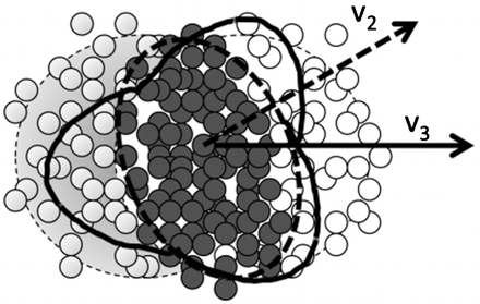
Elliptic and triangular flows from a fluctuating initial state.

Open in new tabDownload slide

Fig. 3.

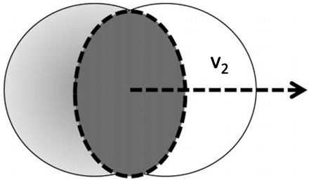
Elliptic flow from a smooth almond-shaped initial state.

Open in new tabDownload slide

Here we make a comment on event-by-event fluctuations in the initial conditions in hydrodynamical models from the point of view of the numerical solution of the hydrodynamical equation. When the hydrodynamical simulation is performed with initial conditions with event-by-event fluctuation, shock-wave capturing schemes should be used to describe the hydrodynamical expansion correctly. Otherwise, the effect of the fluctuation is smeared. It is known that most of the numerical schemes used in the calculations of the time evolution of the quark–gluon plasma do not satisfy this requirement. In other words, they introduce numerical viscosity to a non-negligible extent. In the early stages of RHIC operation, hydrodynamical models gave us certain evidence of the existence of strongly interacting QGP at RHIC and were eventually regarded as the most reliable dynamical models for high energy heavy ion collisions. However, recent high statistical experimental data impose a more rigorous numerical treatment on the hydrodynamical models. We will discuss this issue in detail later in Sect. 4.

2.1 Experimental data and discussion

Among the various kinds of experimental observables, thermal photons are one of the most promising ones for investigation of the initial conditions of hydrodynamic models. The PHENIX Collaboration reported an excess from the superposition of pp collisions in its direct photon measurement at low transverse momentum P_T. This excess follows an exponential distribution, which suggests that thermal equilibrium is achieved [41]. They extract the inverse-slope parameter from the photon spectra in Au+Au |$\sqrt {s}=200$| GeV, T=221±19^stat±19^syst. This value is larger than the critical temperature of the phase transition (∼160 MeV), but it is smaller than the initial temperatures of hydrodynamic models at RHIC, T∼ 300–600 MeV. The value is interpreted as the average temperature in the whole hydrodynamic expansion. Contributions from the hadron phase are also important.

It will be appropriate to point out here the importance of the hydro+micro model as an instrument that relates the initial state condition to the final state observables. For example, very often, final state multiplicities are directly predicted from the initial condition from the color glass condensate picture. For example, when the first LHC multiplicity data came out [42], deviation of the experimental data from the prediction of the color glass condensate picture was found and was regarded as a serious problem. In fact, the system goes through several processes in which entropy and multiplicity change, such as thermalization of the quark–gluon plasma, entropy production in the quark–gluon plasma, hadronization, resonance production in the hadron phase, and their decays. It is thus to be emphasized that understanding of the final state observables requires understanding of the whole period of time evolution in heavy ion collisions. We will come back to this issue in Sect. 6.

3. Hydrodynamical expansion

In the early stages of RHIC operation, only hydrodynamical models were able to explain the strong elliptic flow [43], which was solid evidence of the creation of the strongly interacting QGP at RHIC. However, detailed analyses on experimental data eventually revealed the limitations of hydrodynamical models. They have difficulty in explaining e.g. the elliptic flow at forward/backward rapidity, HBT results, the centrality dependence of elliptic flow, and so forth. At the same time, viscosities became one of the most central topics in relativistic heavy ion collisions, while most analyses had been carried out with ideal hydrodynamics. After the discovery of the strongly interacting QGP, the main interest at RHIC shifted to the understanding of the detailed properties of the strongly interacting QGP.

3.1 Hydrodynamical equations

The basis of hydrodynamical models is energy and momentum conservation,

\begin{equation}\label{eq3.1} \partial_{\mu}T^{\mu \nu}(x) = 0 , \end{equation}

(3.1)

where T^μν(x) is the energy momentum tensor. In the case of an ideal relativistic fluid, the energy momentum tensor is given by

\begin{equation}\label{eq3.2} T^{\mu \nu}(x)= [ \epsilon (x) + p(x) ] u^\mu (x) u^\nu (x) - p(x) g^{\mu \nu}, \end{equation}

(3.2)

where ϵ(x), p(x), and u^μ(x) are the energy density, pressure, and four velocity, respectively. Equation (3.1) is solved numerically simultaneously with the charge conservation relation,

\begin{equation} \label{eq3.3} \partial_{\mu}j^\mu(x) = 0. \end{equation}

(3.3)

When one starts to include the effects of dissipation into relativistic hydrodynamics, one is confronted with a rather complicated situation. One of the difficulties is that the naive introduction of viscosities, first-order theory (i.e., first order in gradients), suffers from acausality. The heat conduction equation allows instantaneous propagation of heat because of its parabolicity. The acausality of first-order hydrodynamics stems from the same reason. In order to avoid this problem, second-order terms in heat flow and viscosities have to be included in the expression for the entropy [44–50], but the systematic treatment of these second-order terms has not been established. Although there has been remarkable progress toward the construction of a fully consistent relativistic viscous hydrodynamical theory, there are still ongoing discussions about the formulation of the equations of motion and about the numerical procedures [51].

The basic tenet that has to be given up in dissipative hydrodynamics is the assumption of a uniquely defined local rest frame. Away from equilibrium the vectors defining the flows of energy, momentum, and conserved charges can be misaligned. We can still define a local rest frame by just choosing a velocity u^μ(x) in the laboratory frame. Then the energy-momentum tensor and the conserved charge current take more general involved forms,

\begin{equation} T^{\mu \nu}(x) = [ \epsilon(x) + p(x)+\Pi(x) ] u^\mu(x) u^\nu(x) - [p(x)+\Pi(x)] g^{\mu \nu} + 2 W^{(\mu} u^{\nu)} + \pi^{\mu\nu},\label{eq3.4}\end{equation}

(3.4)

\begin{equation}j^\mu (x) = n(x) u^\mu + V^\mu,\label{eq3.5} \end{equation}

(3.5)

where V^μ and W^μ are corrections to the flow of conserved charge and energy that are orthogonal to u^μ and T^μνu_ν, respectively, π^μν (with the orthogonality conditions u_μπ^μν=π^μνu_ν=0) is the symmetric traceless shear stress tensor, and Π is the bulk stress. (⋯) indicates symmetrization with regard to the indices. Usually u^μ is chosen to define one of the two standard frames: the Eckart frame where the velocity is given by the physical flow of net charge (then V^μ=0), or the Landau frame where the velocity is given by the energy flow (then W^μ=0). We refer the reader to the article by Muronga and Rischke for further discussions [52].

At first order the new structures are proportional to gradients of the velocity field u^μ, and only three proportionality constants appear: the shear viscosity η, the bulk viscosity ζ, and the heat conductivity κ. With the usual definitions the first-order relations in the Landau frame are [49]

\begin{equation} \Pi = -\zeta \nabla_\mu u^\mu, \label{eq3.6}\end{equation}

(3.6)

\begin{equation}q^\mu = - \kappa \frac{nT^2}{e+p} \nabla^\mu \frac{\mu}{T},\label{eq3.7}\end{equation}

(3.7)

\begin{equation}\pi^{\mu\nu} = 2 \eta \nabla^{<\mu} u^{\nu>},\label{eq3.8} \end{equation}

(3.8)

where q^μ=−(ϵ+p)/n V^μ is the heat flow, ∇^μ=(g^μν−u^μu^ν)∂_ν is the covariant derivative orthogonalized to the flow vector, and T and μ are the temperature and chemical potential for the conserved charge, respectively. Here only one conserved charge is assumed, but the extension to cases with more than two conserved charges is straightforward. 〈⋯〉 refers to the symmetrization of indices with the trace subtracted. The entropy current S^μ receives additional contributions beyond the equilibrium term su^μ and one can show that all three transport coefficients are positive, demanding that the entropy is strictly non-decreasing, ∂_μS^μ≥0.

At second order many more new parameters, related to relaxation phenomena, appear. Currently, most viscous hydrodynamical calculations use the relativistic dissipative equations of motion that were derived phenomenologically by Israel and Stewart [47] and variants of those, while some use the method by Öttinger and Grmela [48–50]; see, e.g., Ref [13]. Recently, second-order viscous hydrodynamics from AdS/CFT correspondence was derived [53], as well as a set of generalized Israel–Stewart equations from kinetic theory via Grad's 14-momentum expansion, which have several new terms [54]. On the other hand, however, a stable first-order relativistic dissipative hydrodynamical scheme was also proposed on the basis of renormalization-group consideration [55,56].

In heavy ion physics, the shear viscosity, in particular its ratio with the entropy density, η/s, has attracted most attention among the three transport constants above. Interesting seminal investigations on the effects of bulk viscosity have begun [57,58], while heat conductivity has still not been investigated systematically in connection with RHIC data. There have also been few systematic investigations into the second-order parameters.

Once the equations of state are given, Eq. (3.1) is solved, the effect of the phase transition being automatically taken into account; this is one of the advantages of the hydrodynamical model. We will discuss this feature in the next subsection. Recently, the lattice(-inspired) equation of state, which is connected to the equation of state of a resonance gas at low temperature, has mostly been used in hydrodynamical models. As the fireball expands, the temperature and density inside become so small that the assumption of the hydrodynamical picture becomes inapplicable. Thus, models with only a hydrodynamical component cannot describe all the stages of relativistic heavy ion collisions from the thermalized quark–gluon plasma stage to kinetic freezeout. One route to such a description is to connect a hydrodynamical simulation to a hadron-based event generator, as discussed in Sect. 6.

3.2 Equation of state and transport coefficients

One of the advantages of hydrodynamical models over other phenomenological models is their direct relation with the equation of state of QCD. Using hydrodynamical models one can directly find the consequence of the phase transition in experimental observables. In hydrodynamical models, historically, the equation of state with a first-order phase transition based on the bag model has been widely used, because of its simplicity and lack of conclusive results on the equation of state of QCD. In recent hydrodynamical calculations, the lattice(-inspired) equation of state has been widely employed, because of the development of thermodynamical analyses based on the first principle calculation, lattice QCD simulation. The equation of state of QCD for 2+1 flavors and also that including the charm quark (2+1+1 flavors) by means of lattice simulations were reported by Borsanyi et al. [59] The HoTQCD Collaboration has investigated the chiral and deconfinement aspects of the phase transition with 2+1 flavors using several kinds of staggered fermions [60]. There were some differences between the two groups in the critical temperature, the temperature dependence of the so-called interaction measure and so on, but gradually the differences are disappearing. At the same time, Wilson fermion simulation has also been applied to the analysis of QCD thermodynamical properties [61]. Quantitative analyses of QCD thermodynamics with the lattice simulation have just started. For conclusive results, improvement in actions, the approach to the continuum limit, simulation at the real pion mass and so on need to be carried out.

Simulations at finite chemical potentials on the lattice suffer difficulties in the execution of Monte Carlo simulations owing to the sign problem in the fermion determinant. Although there have been some developments recently, such as the Taylor expansion method and the reweighting method [62–72], the development in the study of finite chemical potential lattice simulations is relatively slow compared to lattice QCD study at the vanishing chemical potential. Although a lot of attempts have been made to circumvent the problem, we still need a breakthrough to explore the QCD properties in the whole region on the T–μ plane.

In relativistic viscous hydrodynamical models, we need to input more information related to transport coefficients, shear and bulk viscosities, heat conductivity, and relaxation times, besides equations of state. The investigation of the transport coefficients of strongly interacting QGP and hadron gas is one of the most difficult problems in the field. There are several studies on transport coefficients with various approaches: AdS/CFT [53], lattice QCD [73,74], finite temperature perturbative QCD [75–77], microscopic transport models [78–82], and the relativistic quantum Boltzmann approach [83]. However, to reach a conclusive result on the transport coefficients, in addition to theoretical calculations, it is important to extract transport coefficients from comparisons of phenomenological model analyses and experimental data.

3.3 Jet energy loss

One of the most interesting features related to hydrodynamical expansion is jet energy loss. A lot of interesting experimental results that suggest the existence of very large jet energy loss have been reported. To explain these results, the interaction between jets and the medium needs to be understood. At the moment, there are perturbative QCD-based approaches, the higher twist formalism, the AMY formalism, the GLV formalism, the ASW formalism, and the AdS/QCD approach for jet energy loss (for references see, e.g., Ref. [84]).

Despite the large amount of effort put into the development of a perturbative description of the hadron production in heavy ion collisions, there are uncertainties remaining about the exact nature of jet–medium interactions in the kinematic and temperature regimes relevant at RHIC. As a whole, the above four approaches describe the RHIC data well, but they reach very different quantitative conclusions about the quenching strength, or transport coefficient, |$\hat q$|⁠. This does not come as a big surprise, since the approaches differ in some of their basic assumptions, and there are large uncertainties in modeling hard probes beyond the calculation of the energy loss rate for a quark or gluon.

Currently the big picture can be summarized as follows: perturbative calculations under various assumptions are compatible with the RHIC data, but the constraints are insufficient to rule out any of the models. The experimental constraints are also insufficient to completely exclude non-perturbative mechanisms for jet quenching. Calculations using the AdS/CFT correspondence to model strongly interacting QCD [85–87] can describe the same basic phenomenology. Most likely this challenge to perturbative QCD can only be answered at LHC. The extrapolation of jet quenching to larger jet energies is significantly different in strong coupling and perturbative scenarios [88]. It is also possible to assume a small regime of strong non-perturbative quenching around T_c together with perturbative quenching at higher temperatures. Such hybrid scenarios might be hard to distinguish experimentally. One such picture was recently explored by Liao and Shuryak [89]. They found that a “shell”-like quenching profile in which quenching is enhanced around T_c can give better simultaneous fits to single hadron suppression and elliptic flow. For more details, see, e.g., Ref. [84].

3.4 Hydrodynamical expansion

Before moving on to a discussion of experimental data on hydrodynamical expansion, in this subsection we show the behavior of the temperature and chemical potential in hydrodynamical expansion. As an example, we depict the behavior of isentropic trajectories in the T–μ plane for Au+Au |$\sqrt {s_{\mathrm {NN}}}=200$| GeV central collisions in Fig. 4. The dotted line stands for the phase boundary between the QGP and the hadronic phase (note that, due to small baryochemical potentials, the phase boundary is an almost flat line at T_c=160 MeV). In addition to the central cell, we also investigate the isentropic trajectory of a cell close to the surface of the initially produced QGP. Whereas the isentropic trajectory of the central cell located at (0,0,0) starts in the QGP phase (solid line), the cell at the initial surface of the QGP (dashed line) only exhibits an evolution from the mixed phase to the hadronic phase. Both trajectories are terminated at the freezeout temperature, T_f=110 MeV.

Fig. 4.

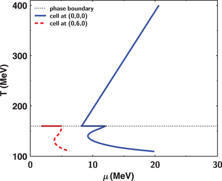
Isentropic trajectories on the T–μ plane in the case of the first-order phase transition. The solid (dashed) line stands for the time evolution of the cell that is located at (x,y,η)=(0,0,0)(=(0,6,0)) at the initial time. The dotted line represents the phase boundary.

Open in new tabDownload slide

3.5 Experimental data and discussion

The calculated results shown in this subsection are based on Ref. [7]. To emphasize the importance of the final state interactions in the freezeout process in understanding hadron observables in relativistic heavy ion collisions, in this subsection we only show the results of the pure hydrodynamical calculation. The calculation is performed with a (3+1)-dimensional ideal hydrodynamical model with a Glauber type initial condition and a bag model equation of state. The effects of final state interactions will be discussed in Sect. 6. This calculation can thus be considered as a baseline for recent more realistic hydrodynamical models.

In the initial energy density distribution, the maximum value of the energy density is 55 GeV/fm³, which is relatively higher than in other hydrodynamical models, because in the pure hydrodynamical calculation we just use a single freezeout temperature and neglect both resonance decays and final state interactions. Usually parameters for the initial condition are set from comparison with experimental data for single particle distributions, rapidity distributions, and P_T distributions in central collisions. Therefore, hydrodynamical models have a predictive power for other physical observables such as collective flow and the impact parameter dependence of various physical observables. We include the small baryon number density in these calculations. The starting time of hydrodynamical expansion is τ₀=0.6 fm. For details of the parameters used in the calculations and the equation of state, see Ref. [7].

First we show two examples that clearly show the limitations of pure hydrodynamical models. One is the P_T spectra of p and multi-strange particles and the other is the elliptic flow as a function of the rapidity. Figure 5 shows the P_T spectra of π, K, and p in Au + Au at |$\sqrt {s_{\mathrm {NN}}}=200$| GeV for central collisions. Our calculation succeeds in reproducing the π spectra measured by PHENIX [90] up to P_T∼2 GeV. However, due to the model assumption of chemical equilibrium down to the (low) kinetic freezeout temperature, we fail to obtain the correct normalization and hadron number ratios, even though the shape of the P_T spectra of p and multi-strange baryons (shown in Fig. 6) is close to that of the experimental data. In order to obtain the proper normalization for the p spectra and hadron number ratios, we adopt a procedure outlined in Refs. [91,92]; it renormalizes the proton P_T spectra using the p to π ratio at the critical temperature. It is straightforward to extend this procedure to hyperons and multi-strange baryons as well, even though we choose to show the raw, unrenormalized, result for the multi-strange baryons in Fig. 6 to elucidate the situation prior to renormalization.

Fig. 5.

P_T spectra for π⁺, K⁺, and p in central collisions with PHENIX data [90]. For the proton we rescale our result using the ratio at the chemical freezeout temperature; see text for details.

Open in new tabDownload slide

Fig. 6.

P_T spectra for multi-strange baryons in central collisions with STAR data [93]. In this pure hydro calculation no additional procedure for normalization has been done.

Open in new tabDownload slide

The need to renormalize the p spectra suggests that the assumption of a persistent chemical equilibrium throughout the hadron phase until kinetic freezeout is not realistic and that an improved treatment of the freezeout process is required. One method to deal with the separation of chemical and thermal freezeout is the partial chemical equilibrium model (PCE): [23,26,94] below the chemical freezeout temperature T_ch one introduces a chemical potential for each hadron whose yield is supposed to be frozen out at that temperature. While the PCE approach can account for the proper normalization of the spectra, it fails to reproduce the transverse momentum spectra and mass dependence of the elliptic flow [95]. In Sect. 6, we shall utilize our hybrid hydro+micro model to decouple the chemical freezeout from the kinetic freezeout. In these hybrid approaches [4,96–98], the freezeouts occur sequentially as a result of the microscopic evolution. Flavor degrees of freedom are treated explicitly through the hadronic cross sections in the microscopic transport, which leads to the proper normalization of all hadron spectra.

Figure 7 shows the elliptic flow as a function of the pseudo-rapidity η in central (3–15%) and mid-central collisions (15–25%). In both cases our hydrodynamical model calculations overestimate the elliptic flow at forward and backward pseudo-rapidities, similar to the results shown in Ref. [23]. At large forward and backward rapidities the assumptions of perfect hydrodynamical models, such as local equilibrium, vanishing mean free path, and negligible viscosity effect, are apparently no longer valid. The difference between the experimental data and calculated results at forward and backward rapidities increases with the impact parameter, implying a decrease of the volume in which the hydrodynamical limit is achieved.

Fig. 7.

Elliptic flow as a function of η with PHOBOS experimental data [99] for central (3–15%) and mid-central (15–25%) collisions. Impact parameters are set to 4.5 (central) and 6.3 (mid-central) fm, respectively.

Open in new tabDownload slide

Next we move on to the topic of jet energy loss in an expanding hydrodynamical medium as an interesting application of the hydrodynamical model. Figure 8 shows the results from a comparative study by Bass et al. at RHIC [101]. Jets are propagated through a medium described by the same hydrodynamics, using three different schemes for energy loss: ASW, higher twist (HT), and AMY. Figure 8 shows R_AA as a function of P_T for two different centrality bins. It shows that the P_T-dependence and the centrality dependence of R_AA are described well by all three models. Each model has one free parameter that has been adjusted: the strong coupling α_S in AMY, |$\hat {q}_0$| for the overall fit parameter in HT, and K (⁠|$\hat {q} =K \cdot 2 \cdot \epsilon ^{3/4} $|⁠) in ASW. These parameters are fixed from the comparison with R_AA data in central collisions (the top figure in Fig. 8).

Fig. 8.

R_AA as a function of P_T for central (top) and mid-central (bottom) collisions calculated from the ASW, higher twist, and AMY energy loss models. The single parameter in each model has been fitted to describe the data by PHENIX [100].

Open in new tabDownload slide

This study confirms the remarkably large |$\hat q$| in the ASW model compared to that in the HT approach. For the case where the quenching strength scales with ϵ^3/4, the initial values |$\hat q_0$|² found for the quark at the center of the fireball in a central collision are [101]

\begin{equation}\label{eq3.9} \begin{cases} \hat q_0 = 18.5\>\text{GeV}^2/\text{fm for ASW}, \\ \hat q_0 = 4.5 \> \text{GeV}^2/\text{fm for HT} \end{cases} \end{equation}

(3.9)

and for the case where the quenching strength scales like the temperature T they are

\begin{equation}\label{eq3.10} \begin{cases} \hat q_0 = 10\>\text{GeV}^2/\text{fm for ASW}, \\ \hat q_0 = 2.3\> \text{GeV}^2/\text{fm for HT}, \\ \hat q_0 = 4.1\> \text{GeV}^2/\text{fm for AMY} . \end{cases} \end{equation}

(3.10)

Note that the jet propagation in AMY model is calculated self-consistently as a function of the local temperature so that there is no difference between the two cases.

This comparison is unique and very valuable in the respect that the same initial hard cross sections and the same maps for the fireball, from the same (3+1)-dimensional ideal hydrodynamics, were used. Any differences in the extracted values of |$\hat q$| are solely due to differences in models for the jet energy loss. One of the conclusions is that our current knowledge applied to R_AA leaves a rather large uncertainty in the determination of |$\hat q$|⁠.

Here we make a short comment on the jet energy loss at LHC. The ALICE Collaboration reported the nuclear modification factors R_AA as a function of P_T of charged particles in central and peripheral Pb–Pb collisions at |$\sqrt {s_{\mathrm {NN}}}=2.76$| TeV [102]. They found that, in central collisions, R_AA is more suppressed up to P_T=7 GeV compared to the PHENIX and STAR experiments at RHIC, which suggests that a much denser medium is produced and stronger parton energy loss occurs at LHC. R_AA decreases with P_T for 2<P_T<7 GeV, takes a minimum around P_T=7 GeV, and, interestingly, increases with P_T for P_T>7 GeV. The increase of R_AA at high P_T was observed for the first time at LHC. It was not seen clearly at RHIC.

4. Numerical schemes for solving hydrodynamical equations

In this section, we first explain the current status of hydrodynamical models from the point of view of numerical schemes for relativistic hydrodynamical equations. As we showed in Tables 1 and 2, hydrodynamical models are categorized into ideal and viscous versions. In addition, the difference of each hydrodynamical model is found in the space-time dimension of simulation, initial conditions, equations of state, and prescriptions for the freezeout process. In current understanding, the most realistic hydrodynamical model should have the following features: viscosity effects, (3+1)-dimensional space-time expansion, event-by-event fluctuating initial conditions, lattice QCD-inspired equations of state, and a freezeout process that is described by hadron-based cascade models. On these issues, ideal hydrodynamical models have been studied more deeply and their status is considered to be more mature than viscous hydrodynamical models. The investigation with viscous hydrodynamical models has just started.

In addition to the above issues, an important ingredient in hydrodynamical models should be seriously taken into account. It is the choice of which numerical scheme to adopt for solving the relativistic hydrodynamical equation. Up to now, only a little attention has been paid to this point. As long as we analyze multiplicities and collective flow using smoothed initial conditions, the choice of numerical scheme is not so important. However, when we start to investigate viscosity effects and event-by-event fluctuations, we need to choose suitable numerical schemes carefully.

The relativistic hydrodynamical equation is a nonlinear system equation, whose analytical solution is usually difficult to find. However, from the one-dimensional wave equation ∂_tu+c∂_xu=0, which is much simpler than the actual relativistic hydrodynamical equation, we can explore a suitable numerical scheme by comparing with the analytical solution. A naive differential scheme such as the FTCS (forward-time central-space) scheme (⁠|$u^{n+1}_j=u^n_j - \frac {1}{2} \nu (u^n_{j+1}-u^n_{j-1}$|⁠) ³, with |$\nu =c\frac {\Delta t}{\Delta x}$|⁠) causes an unphysical oscillation, which continues to grow after several time steps. In order to stabilize the unphysical oscillation in the FTCS scheme, one can use e.g. the Lax–Friedrich scheme. In this scheme |$u^n_j $| on the right hand side of the FTCS scheme is replaced by the averaged value |$\frac {1}{2}(u^n_{j-1}+ u^n_{j+1})$|⁠. This scheme is stable if the Courant–Friedrichs–Lewy condition (CFL condition) (|ν|<1) is satisfied, but it is known that it suffers huge numerical dissipation. In other words, the average manipulation introduces artificial viscosity. An improved version of the Lax–Friedrich scheme is the Lax–Wendroff scheme, which has second-order accuracy in time and space,

\begin{align*} u^{n+1/2}_{j+1/2} & = \frac{u^n_{j+1}+ u^n_j}{2} - \frac{1}{2}c\frac{\Delta t}{\Delta x} (u^n_{j+1}-u^n_j), \\ u^{n+1}_j & = u^n_j - c\frac{\Delta t}{\Delta x} (u^{n+1/2}_{j+1/2}-u^{n-1/2}_{j-1/2}). \end{align*}

This scheme is stable, but the unphysical oscillation occurs at discontinuity. In order to avoid this problem, it is necessary to introduce artificial viscosity or flux limitation. In conjunction with this fact, we cite Godunov's theorem: no second-order or higher-order explicit monotonous scheme exists. A systematic discussion on numerical schemes is beyond the scope of this article; for details, please see, e.g., Ref. [103]. From these lessons for numerical schemes for the wave equation, we can deduce those for the relativistic hydrodynamical equation, though actual numerical tests are indispensable. i) First-order accuracy scheme: For stability at discontinuity some average manipulation is needed, but this introduces large dissipation. ii) Second-order accuracy: To remove the numerical oscillation at discontinuity, one needs artificial viscosity or a flux limiter. The former suggests that a simple central difference scheme of the first-order accuracy might have a large artificial viscosity, which is crucial for the study of the viscosities of matter created in relativistic heavy ion collisions.

For event-by-event fluctuating initial conditions, shock-wave capturing schemes play an important role in dealing with discontinuity in the initial conditions. A lot of shock-wave capturing schemes have been proposed and developed. On the other hand, in relativistic heavy ion collisions, the SHASTA, rHLLE, and KT algorithms are mainly used. In particular, the SHASTA algorithm, which is widely used in the study of relativistic heavy ion collisions, is known as the first version of the flux corrected transport (FCT) algorithm [104]. In this algorithm, a low-order solution is calculated first. It incorporates a large numerical diffusion effect. In the second step, as much diffusion as possible is removed from the low-order solution. The amount of antidiffusion fluxes is determined with the mask coefficient A_ad. This default value is A_ad=1, which can be set to lower values to reduce the amount of antidiffusion. In Ref. [105] an interesting demonstration of the interplay between the numerical viscosity and physical viscosity was shown. A comparison was made with numerical solutions of the Riemann problem, one with the standard mask coefficient A_ad=1.0 SHASTA with a small physical viscosity η/s=0.01 and the other with a reduced mask coefficient A_ad=0.8 SHASTA with vanishing viscosity. It was found that the difference between the two numerical calculations is very small, which implies that it might be difficult to distinguish between the physical viscosity and the artificial dissipation. For quantitative investigation of the viscosities in the quark matter, one needs to estimate the amount of artificial viscosity existing in numerical schemes carefully or choose numerical schemes known to have less artificial viscosity. Furthermore, in Ref. [105], a comparison between the different shock-wave capturing schemes, the SHASTA, KT, and NT schemes, was made and found that all the algorithms reproduce the analytic solution with nearly the same accuracy and numerical artifacts (Figs. 9 and 10).

Fig. 9.

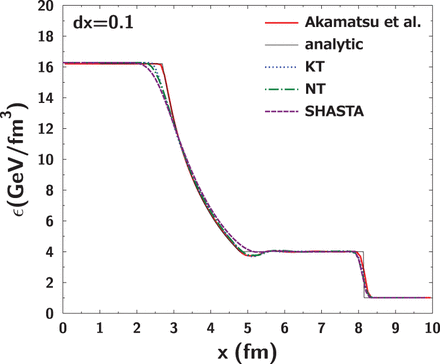
Energy density distributions as a function of x from numerical results (SHASTA (short-dashed line), KT (dotted line), NT (long-dashed line), and Akamatsu et al. (to be published) (red solid line)) together with the analytic Riemann solution.

Open in new tabDownload slide

Fig. 10.

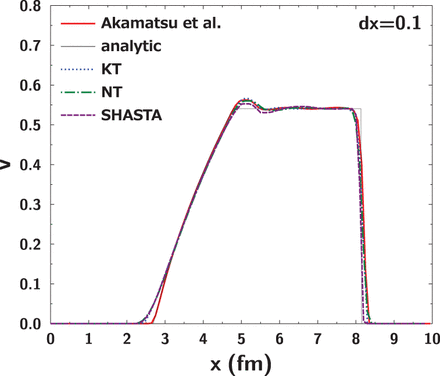
Velocity distributions as a function of x from numerical results (SHASTA (short-dashed line), KT (dotted line), NT (long-dashed line), and Akamatsu et al. (to be published) (red solid line)) together with the analytic Riemann solution.

Open in new tabDownload slide

Recently, Akamatsu et al. proposed a fast numerical scheme (Y. Akamatsu et al., to be published) for causal relativistic hydrodynamics with dissipation for analyses of relativistic high energy collisions, which is based on Ref. [106]. In the numerical scheme, Israel–Stewart theory was adopted and the Israel–Stewart equations were decomposed into the inviscid part and the dissipative part. For the inviscid part a relativistic Riemann solver [107–115] is used and for the dissipative part the piecewise exact solution method [116–118] is employed in order to achieve less artificial dissipation and less computational time. Riemann solvers are numerical fluid dynamical solvers that are based on the concept of the Riemann problem. Several kinds of Riemann solvers have been proposed: the Godunov method, the Roe scheme, HLLE and HLLC solvers, and so on. Each solver has advantages and disadvantages in numerical cost, calculational accuracy, and coding complexity [103,107]. In order to obtain the correct physical viscosity, for the inviscid part as well as the dissipative part, we need to choose numerical schemes that suffer as little artificial dissipative effect as possible. For the inviscid part, Y. Akamatsu et al. (to be published) use the relativistic Godunov method, which is based on the exact solution of the Riemann problem. Figures 9 and 10 show numerical solutions of the relativistic Riemann problem for an ideal fluid on a grid with N_x=100 cells with Δx=0.1 fm after N_t=100 time steps at t=4 fm together with the analytic solution. The initial conditions are set to be the same as those in Ref. [105]. On the left, the initial temperature is T₀=0.4 GeV and, on the right, T₀=0.2 GeV; the energy density ϵ is given by |$\epsilon =\frac {3g}{\pi ^2}T^4$| (g=16). The numerical results for the SHASTA, KT, and NT schemes are taken from Ref. [105]. The SHASTA, KT, and NT schemes reproduce the analytic Riemann solution with nearly the same accuracy and numerical artifacts. On the other hand, we can see that the red line (Y. Akamatsu et al., to be published) is closer to the analytical solution around x=3 fm, which implies that this scheme suffers a smaller artificial dissipative effect and is more suitable for physical viscosity analyses. A comparison of rHLLE and SHASTA was done in Ref. [119]. It was found that rHLLE has almost the same artificial viscosity as SHASTA.

5. Hadronization

In hydrodynamical models the hadronization process from the QGP phase to the hadron phase is naturally encoded in the equation of state. At RHIC, hydrodynamical calculations do well for explaining a lot of experimental data, the P_T spectra, and the elliptic flow up to P_T∼ 2 GeV. However, above P_T∼2 GeV the results from hydrodynamical models start to show deviation from experimental data, which suggests that other mechanisms become dominant at higher P_T instead of the hydrodynamical feature. In the intermediate P_T (2≤P_T≤6 GeV) the recombination mechanism is dominant and at high P_T (≥6 GeV) the fragmentation mechanism plays an important role. These transverse momentum regions where the hydrodynamical picture, recombination model, or fragmentation mechanism works well depend on collision energy. For example, at LHC the hydrodynamical description may work up to P_T∼4−5 GeV [33]. There have been attempts to use thermodynamical properties that are described with a hydrodynamical model as inputs for the recombination model and fragmentation mechanism [120,121]. It may become possible to construct more realistic dynamical models to understand the physics of relativistic heavy ion collisions by employing the recombination model and fragmentation process for hadronization in a hydrodynamical model. In the next subsection, we give a brief description of the recombination model.

5.1 Recombination model

Quark recombination or coalescence is the best candidate for the physical mechanism to explain a large amount of experimental data at intermediate P_T at RHIC. Currently, not only at LHC but also at relatively low collision energy experiments, analyses with the recombination picture are ongoing [122]. First the quark number scaling law was found in the behavior of elliptic flow as a function of the transverse momentum, which is considered to be a signature of quark recombination. For a quark phase with the elliptic flow |$v_2^q(P_T)$| at the time of hadronization, simple instantaneous recombination models predict

\begin{equation}\label{eq5.1} v_2^H(P_T) = n v_2^q\left(\frac{P_T}{n}\right)\!, \end{equation}

(5.1)

where n is the number of valence quarks. This scaling law describes the key feature of experimental data at intermediate P_T notably well.

Generally, recombination models assume a universal phase space distribution of quarks at hadronization. Quarks turn into baryons, qqq→B, and mesons, |$q\bar q\to M$|⁠. These processes are described either by using instantaneous projections of quark states onto hadron states [123–127], or dynamical coalescence processes with finite width hadrons governed by rate equations [128]. Note that usually only the valence quarks of the hadron are taken into account although generalization has been attempted [127].

The original instantaneous projection models explicitly preserve only three components of the energy-momentum four-vector in the 2→1 and 3→1 processes. The yield of mesons can be expressed through convolution of the Wigner function W_ab for a pair of partons, a and b, and the Wigner function Φ_M encoding the meson wave function:

\begin{equation}\label{eq5.2} \frac{dN_M}{d^3 P} = \int \frac{d^3 R}{(2\pi)^3} \sum_{ab} \int \frac{d^3q d^3r}{(2\pi)^3} W_{ab}\left(\mathbf{R}+\frac{\mathbf{r}}{2}, \frac{\mathbf{P}}{2}+\mathbf{q} ; \mathbf{R}-\frac{\mathbf{r}}{2}, \frac{\mathbf{P}}{2}-\mathbf{q} \right) \Phi_M(\mathbf{r},\mathbf{q}). \end{equation}

(5.2)

The quark Wigner functions are usually approximated by classical phase space distributions. Hadron spectra at intermediate P_T are described well by considering the factorization of W_ab into thermal quark distributions: [124],

\begin{equation}\label{eq5.3} W_{ab}\left(\mathbf{r}_1,\mathbf{p}_1;\mathbf{r}_2,\mathbf{p}_2\right) = f_a\left(\mathbf{r}_1,\mathbf{p}_1\right) f_b(\mathbf{r}_2,\mathbf{p}_2). \end{equation}

(5.3)

Correlations between quarks can be introduced to model correlations found between hadrons [129] without interfering with the excellent description of the spectra and hadron ratios.

The strength of the quark recombination picture is in its predictive power, which originates from its explaining all measured hadron spectra at intermediate P_T, basically with one parameter for the quark distribution function at hadronization. It has been shown that at low momenta resonance recombination is compatible with hydrodynamics and kinetic equilibrium [130], but on the other hand, because thermalized states do not retain memories of previous time, all phenomena with long time scales in the equilibrated region should be expected to be described by hydrodynamics. They include the quark number and kinetic energy scaling observed at RHIC at low momenta [130]. The possibility of including quark recombination explicitly in the hydrodynamical model has been studied in Refs. [120,121].

5.2 Experimental data and discussion

Using the recombination model, we can explore the production of quark soup, which is a consequence of the QCD phase transition. After the success of the recombination model at RHIC, the scaling property of the elliptic flow has been tested over a wide range of collision energy to investigate the properties of the strongly interacting QGP. The elliptic flows of π^±,p, and Λ were measured in Pb+Pb collisions at |$\sqrt {s_{NN}}=17$| GeV at SPS by NA49 [131]. They found that the quark number scaling in the elliptic flows of these particles holds in the P_T range covered by the data (up to P_T/n≈1 GeV; see Fig. 6 in Ref. [131]). Since P_T is limited to rather low values, however, this should not be viewed as a conclusive test for the quark recombination mechanism at SPS.

At LHC, analyses of the quark number scaling in the elliptic and triangular flows of identified particles have just started. In Ref. [132], ALICE shows the elliptic and triangular flows per constituent quark of π^±,K^±, and |$\bar {p}$| as a function of the transverse kinetic energy (KE_T) per quark for more central (10–20%) and more peripheral (40–50%) Pb+Pb collisions at |$\sqrt {s_{NN}}=2.76$| TeV. They report that, within errors, the flows of π and K follow the scaling, while the flow of |$\bar {p}$| deviates in the more central and more peripheral events. In the triangular flow they find the same feature as in the elliptic flow, i.e., the triangular flow of |$\bar {p}$| shows deviations from the KE_T scaling. However, this investigation was done in a relatively low transverse kinetic energy region (KE_T/n<1 GeV) where hydrodynamical behavior is expected to be dominant. Therefore, this deviation from the KE_T scaling in the elliptic and triangular flows could be explained by mass splitting and mass ordering realized by hydrodynamical motion. To obtain a conclusive result for the quark number scaling in the collective flow at LHC, measurement at higher transverse kinetic energy, where the effects of the recombination mechanism are more clearly observed, is indispensable.

For experimental confirmation of the quark number scaling in the elliptic flow, no particles are more important than the ϕ meson. Because it is composed of one quark and one antiquark and its mass is close to that of the proton, analyses of the elliptic flow of ϕ reveal the dominant process in hadronization at intermediate P_T: the recombination mechanism or thermal process as described by hydrodynamics [133]. In addition, because multi-strange hadrons have large mass and small hadronic cross sections, they should be less sensitive to hadronic rescattering in the later stage of collisions and be a good probe for the early state of collisions such as partonic elliptic flow. The STAR Collaboration measured the v₂ of multi-strange hadrons (ϕ,Ξ, and Ω) in Au+Au collisions at |$\sqrt {s_{\mathrm {NN}}}=200$| GeV and showed that the quark number scaling works in the elliptic flow of multi-strange hadrons [134]. This implies that the partonic collectivity is built up at the top RHIC energy.

Furthermore, the STAR Collaboration investigated the energy dependence of the elliptic flow as a function of the transverse momentum for ϕ at RHIC [135]. The quark number scaling in the elliptic flows of π, K, p, Λ, and Ξ works well at both |$\sqrt {s_{NN}}=39$| and 11.5 GeV in Au+Au collisions. They found that, while at |$\sqrt {s_{NN}}=39$| GeV the elliptic flow of ϕ also follows the quark number scaling, at |$\sqrt {s_{NN}}=11.5$| GeV the elliptic flow per constituent quark of ϕ is much smaller than those of the other particles. Only the ϕ meson is out of the quark number scaling of the elliptic flow at this energy. They conclude that this indicates the dominance of hadronic interactions with the decrease in the beam energy. To confirm this, measurement of the elliptic flow of Ω would be helpful.

At the top RHIC energy, the elliptic flow of hadrons that contain only light flavor quarks (u, d, and s) follows the quark number scaling. Does the quark number scaling work in the elliptic flow of hadrons that are composed of heavy flavors? A recent STAR measurement of the elliptic flow of J/ψ gives the answer to this question. It shows that the elliptic flow of J/ψ is consistent with zero over the measured P_T range, which is significantly smaller than that of ϕ and inclusive charged hadrons [136]. The picture of J/ψ production being dominated by charm quark recombination with significant charm quark flow is disfavored. On the other hand, the elliptic flow of open charm mesons is well understood by the recombination of a light (anti)quark and an (anti)charm quark with elliptic flow [137].

Next we argue that the recombination model is a powerful tool to understand hadron properties and the QCD phase diagram with high energy heavy ion collisions. The investigation of the elliptic flow of hadron resonances with the recombination picture at RHIC makes it possible to understand final state interactions in the freezeout processes and the structure of resonances [138]. In principle, there are two different mechanisms that contribute to resonance production and, as a result, there are two types of resonances: (1) primordial resonances—resonances produced from hadronizing the quark–gluon plasma (the QGP mechanism), and (2) secondary resonances—resonances produced in the hadronic final state via hadron–hadron scattering (the HG mechanism). For example, in the case of K*₀, which is composed of d and |$\bar {s}$| quarks, K*₀ is produced by recombination of the d and |$\bar {s}$| quarks in the QGP mechanism, while it is created via scattering of K and π in the HG mechanism. The recombination model tells us that the scaling constant n of the elliptic flow of a hadron species is given by the number of constituent quarks that participate in the production of the hadron: in the case of the QGP mechanism n=2, and in the case of the HG mechanism n=4. From these two contributions the measured elliptic flow is given by

\begin{equation}\label{eq5.4} v_2^{\mathrm{measured}} = r(P_T)v_2^{\rm QGP}+ (1-r(P_T))v_2^{\rm HG}, \end{equation}

(5.4)

where r(P_T) is the fraction of resonances which are produced at hadronization and whose decay products escape from the hadron phase without rescattering. With r(P_T) one can investigate the cross sections of resonances in the hadronic medium. STAR attempted to extract the scaling constants (or apparent constituent quark number) from the measured elliptic flow of K^0* to investigate its production mechanism. Unfortunately, the obtained value of n is n=3±2 [139], from which we cannot draw a definite conclusion. This method is easily extended to explore the structure of exotic hadrons, such as the tetraquark and pentaquark. Utilizing the scaling law of elliptic flow, one can obtain information on the structure of exotic hadrons, whether they have a compact structure or are more like molecular bound states [138].

We can explore the consequences of diquark and quark–antiquark clustering above the deconfinement temperature with event-by-event net charge fluctuations [140]. Recently, lattice QCD calculations have shown that charmonia survive even well above the critical temperature [141–144], which suggests the possibility that hadronization occurs via recombination of not only single q or |$\bar {q}$| but also qq or |$q\bar {q}$|⁠. The D measure, the net charge fluctuation normalized by the entropy, is defined by

\begin{equation}\label{eq5.5} D=4\langle (\Delta Q)^2\rangle/N_{\mathrm{ch}}, \end{equation}

(5.5)

where 〈(ΔQ)²〉 denotes the event-by-event net charge fluctuation within a given rapidity window Δy and N_ch is the total number of charged particles emitted in this window. For a free plasma of quarks and gluons D≈1, whereas for a free pion gas D≈4. However, experimental data at RHIC are rather close to the value for hadron gas, D=2.8±0.05 in central Au+Au collisions at |$\sqrt {s_{NN}}=130$| GeV (STAR) [145,146] and D≈3 (PHENIX) [147,148]. In the recombination scenario, the fluctuation of the net charge |$Q=\sum _iq_i n_i$| is given as

\begin{equation}\label{eq5.6} \langle \delta Q^2 \rangle \equiv \langle Q^2 \rangle - \langle Q \rangle ^2 = \sum_i(q_i)^2 \langle n_i \rangle + \sum_{i,k}c^{(2)}_{ik} \langle n_i \rangle \langle n_k \rangle q_i q_k, \end{equation}

(5.6)

where |$c^{(2)}_{ik}$| are the normalized two-particle correlation functions. In the absence of two-particle correlations, Eq. (5.6) can be rewritten as |$\langle \delta Q^2\rangle = \frac {4}{9} (N_u + N_{\bar u}) + \frac {1}{9}(N_d + N_{\bar d} + N_s + N_{\bar s}) $|⁠, where N_i=〈n_i〉 denotes the average number of the constituent quarks with flavor i. Together with the statistical hadronization model and the experimental values of multiplicity, the net charge fluctuation in the quark recombination scenario is d〈δQ²〉_q/dy=331±27, which is close to the experimental value d〈δQ²〉_had/dy=368±33 [145,146]. Furthermore, the difference in the net charge fluctuations between the quark recombination and the experimental data suggests the necessity of improvement on both the theoretical and experimental sides. One such possibility is to include qq and |$q\bar {q}$| pairs in the hadronization mechanism [140]. If the qq pair and |$q\bar {q}$| are taken into account, Eq. (5.6) is extended to

\begin{equation}\label{eq5.7} \langle \delta Q^2 \rangle = \sum_i (q_i)^2 (N_i + N_{\bar{i}}) + \sum_{ij}(q_i + q_j)^2 \langle n_{ij}\rangle + \sum_{ij} (q_i - q_j)^2 \langle \bar{n}_{ij}\rangle, \end{equation}

(5.7)

where the average numbers of diquarks and |$q\bar {q}$| are proportional to the products of the individual quark numbers: |$\langle n_{ij}\rangle =\alpha (N_i N_j + N_{\bar {i}}N_{\bar {j}})$|⁠, |$\langle \bar {n}_{ij}\rangle \ = \beta N_iN_{\bar {j}}$| with relative pairing weights α and β. They showed that experimental data can be fitted with an appropriate choice of α and β.

In Ref. [140], the problem of the gluonic degrees of freedom was also discussed. According to recent lattice calculations [59–61], the phase transition at small baryon chemical potential is a crossover. This means that the hadronization at RHIC and LHC does not take place from a system where quarks and gluons are active degrees of freedom, but from a state with reduced entropy density. So far, no method on the lattice has been found to identify what the active degrees of freedom in the crossover region are. In Ref. [140] it was shown that entropy density data on the lattice are not inconsistent with those of a gas of constituent quarks, which is assumed in the recombination model. The success of the recombination model strongly suggests that the gluonic degrees of freedom disappear first when the temperature is decreased from well above the (pseudo-)critical temperature. However, it is needless to say that it is important to find a way to identify how the active degrees of freedom change across the crossover region on the lattice in order to steady this picture.

6. The freezeout process

As fireballs expand, the temperature and density inside them become small. Finally the mean free path among particles inside the fireballs becomes so large that the assumption for the hydrodynamical picture becomes invalid. Currently, two separate freezeout processes are believed to occur successively in heavy ion collisions. One is chemical freezeout, at which the ratios of hadrons are fixed, and the other is thermal (kinetic) freezeout, at which the particles stop interacting. Recently, final state interactions between the two freezeout processes have also been included in hydrodynamical models by connecting hadron-based event generators to hydrodynamical calculations. In this picture, kinetic freezeout is found to be not an instantaneous process but a continuous one, as we show in the following.

6.1 Chemical freezeout and thermal freezeout

The chemical freezeout temperature and baryon chemical potential are extracted with the statistical model on the basis of grand canonical formalism. Surprisingly, statistical models are in excellent agreement with experimental data for hadron ratios in a wide range of collision energy from SIS to RHIC [149]. At present the (pseudo-)critical temperature suggested from the latest lattice calculation is T_c=150−160 MeV (see Subsect. 3.2), which is relatively low from the point of view of the statistical model [150]. For example, using a statistical model, Andronic et al. extract the chemical freezeout temperature T_ch=160−166 MeV for LHC Pb+Pb collisions at |$\sqrt {s_{\mathrm {NN}}}=2.76 $| GeV. It might be too early to take lattice results at face value, but this suggests that the physical meaning of the temperature and chemical potential obtained by the statistical model needs to be reexamined. At the same time, one needs to make it clear why the statistical model works very well not only in a wide range of collision energies from SIS to LHC but also for smaller systems such as p+p collisions [151].

At the thermal freezeout temperature, the mean free paths of the hadrons have grown to the order of the system size and the hydrodynamical description, which requires a very small mean free path, is clearly no longer applicable. A first naive guess for the kinetic freezeout temperature T_f would be of the order of the pion mass (∼140 MeV). In practice, the value of the kinetic freezeout temperature in hydrodynamical models is determined from comparison with data of P_T spectra.

The task at the end of a hydrodynamical calculation is to populate fluid cells with particles with the final temperature and flow. For calculations of single particle spectra, the simple assumption of a sudden freezeout process at a certain proper time for each fluid cell is often adopted, neglecting the reverse process from particles to the hydrodynamical medium. Under this assumption, the Cooper–Frye formula [152] is widely used:

\begin{equation}\label{eq6.1} E\frac{dN}{d^3P} = \sum_h\frac{g_h}{(2\pi)^3} \int_\Sigma d\sigma_\mu P^\mu \frac{1}{\exp[(P_\nu u^\nu-\mu_f)/T_{\mathrm{f}}]\pm 1}, \end{equation}

(6.1)

where g_h is the degeneracy factor of the hadron h, T_f and μ_f are the freezeout temperature and baryon chemical potential, respectively, and +(−) is for fermions (bosons). dσ_μ is obtained by calculating the normal vector on the freezeout hypersurface Σ. Once these quantities are given, using Eq. (6.1), one can calculate the distribution of any particle after freezeout.

More realistic models have been investigated. One of them is the continuous emission model (CEM), in which particles are emitted continuously from the whole expanding volume of the system at different temperatures and different times [153]. In the early days of hydrodynamics only kinetic freezeout was implemented. Indeed, at lower collision energies such as at SIS and AGS, the separation between the chemical and kinetic freezeout points is not large on the T–μ plane. However, at RHIC there is a significant difference between kinetic freezeout temperatures from hydro-inspired models and the chemical freezeout temperature from the statistical model. [154]. This fact also manifests itself through the failure to get the correct absolute normalization of some P_T spectra, e.g., that of protons in hydrodynamical calculations, with only a kinetic freezeout [155]. For these reasons, attempts to model separate freezeout processes consistently via modified equations of state were started [23,94,156,157].

6.2 Final state interactions

It turns out that some experimental data are still not understood in a satisfactory way even with the two separate freezeouts. For example, mean transverse momentum 〈P_T〉 as a function of particle mass does deviate from the linear scaling law, which suggests significant final state interactions in the hadronic phase [7]. To explain these effects, and to account for the apparently large viscosities in the hadronic phase, as discussed before, hydro+cascade hybrid models were introduced. They use a hydrodynamical computation of the expansion and cooling of hot QCD bulk matter, and then couple the output consistently to a hadron-based transport model in order to take account of the final state interactions. Pioneering work on hydro+cascade hybrid models was done by Bass et al. [158] using UrQMD. Similar investigations were carried out in Refs. [4,24]. Figure 11 shows a schematic sketch of the hydro + UrQMD model [7]. At the switching temperature T_SW, the mean free path of hadrons becomes so large that the hydrodynamical picture becomes inapplicable. Thus, after this point, the motion of hadrons is described by UrQMD. In practice, at T_SW, hadron distributions are calculated with the Cooper–Frye formula in the fluid and the initial state of UrQMD is produced with them through Monte Carlo methods. Then the UrQMD simulation is started. The reverse process from UrQMD to fluid dynamics is neglected in the simulation.

Fig. 11.

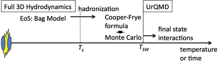
Schematic sketch of the 3D hydro + UrQMD model. T_c and and T_SW are taken to be 160 MeV and 150 MeV, respectively.

Open in new tabDownload slide

6.3 Experimental data and discussion

The main purpose of our hydrodynamical model + hadron-based event generator is to handle realistic final state interactions in the freezeout process. We need to choose an appropriate hadron-based event generator for it. Hadron-based event generators have been developed to understand experimental data especially at lower energy heavy ion collisions. Here we use the UrQMD model for the description of final state interactions in the hadron phase. It gives us reasonable hadron yields, single particle spectra and so on, and it is often used for understanding the baseline of experimental data of relativistic heavy ion collisions.

Here we make a comment on the applicability of cascade models for the description of the afterburner of hydrodynamical models. Recent lattice calculations (Ref. [59]) suggest that the hadron phase is well described as a hadron resonance gas up to the vicinity of the phase transition. Thus, cascade models are, in general, ideal machinery to investigate its time evolution and freezeout process.

If the final state interactions are implemented properly, hydrodynamical models acquire more predictive power for experimental observables. We will show this by comparing single particle spectra and elliptic flows with experimental data. In this subsection we show results calculated with the same initial conditions and equation of state as in pure hydrodynamical calculations: Glauber type initial conditions and a bag model equation of state. In this case the maximum value of initial energy density is 40 GeV/fm³, which is smaller than that of the pure hydrodynamical model, because the inclusion of resonance decays and final state interactions in hydrodynamical models increases particle multiplicity.

First let us consider the argument on the multiplicity, which we mentioned in Sect. 2. We take π⁺ as an example, because it is one of the most dominant particles in the charged hadron multiplicity and is affected a great deal by resonance decays. Figure 12 shows the pseudo-rapidity distributions of π⁺ from the fluid at T_sw (solid line), that from the fluid plus resonance decay effects (open circles), and its final state multiplicity (solid circles). We find that the resonance decay effect is huge and that the multiplicity including the resonance decay effect (open circles) becomes almost twice that of hydro at T_sw (solid line). Furthermore, the additional gain from final state interactions is seen. This result clearly shows that the dynamics of the hadron phase, such as resonance decays and final state interactions, is also important in high energy heavy ion collisions. In short, final state multiplicities cannot be predicted by determining the initial state only.

Fig. 12.

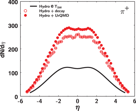
Pseudo-rapidity distribution of π⁺ from hydro at T_sw (solid line), hydro + decay (open circle), and hydro + UrQMD (solid circle) in Au+Au |$\sqrt {s_{NN}}=200$| GeV central collisions.

Open in new tabDownload slide

Figure 13 shows the P_T spectra of π⁺, K, and p in central collisions at |$\sqrt {s_{NN}}=200$| GeV. The most remarkable feature, compared to the pure hydrodynamical calculation, is that the hydro+micro approach is capable of accounting for the proper normalization of the spectra for all hadron species without any additional correction, as is performed in the pure hydrodynamical model. The introduction of a realistic freezeout process therefore provides a natural solution to the problem of separation of the chemical and kinetic freezeouts in the pure hydrodynamical calculation. Similar results have been obtained previously in 1+1- and 2+1-dimensional implementations of the hydro+micro approach [96,159].

Fig. 13.

Comparison of the calculated P_T spectra for π⁺, K⁺, and p in central collisions with PHENIX data [90]. The points are not renormalized.

Open in new tabDownload slide

In Fig. 14 we analyze the P_T spectra of multi-strange particles. Our results show good agreement with experimental data for Λ, Ξ, and Ω for centralities 0–5% and 10–20%. In this calculation no additional procedure for normalization is needed. Recent experimental results suggest that, at the thermal freezeout, multi-strange baryons exhibit weaker transverse flows and higher temperatures closer to the chemical freezeout temperature compared to non- or single-strange baryons [160,161]. This behavior can be understood in terms of the flavor dependence of the hadronic cross section, which decreases with increasing strangeness content of the hadron. The reduced cross section of multi-strange baryons leads to a decoupling from the hadronic medium at an earlier stage of the reaction, allowing them to provide information on the properties of the hadronizing QGP less distorted by hadronic final state interactions [159,162,163]. It should be noted that analogous behavior has already been observed in experiments at CERN SPS [164–168].

Fig. 14.

Calculated P_T spectra of multi-strange particles at centralities 0–5% and 10–20% and STAR data [160].

Open in new tabDownload slide

In Fig. 15 the mean transverse momentum 〈P_T〉 as a function of the hadron mass is shown. Open symbols denote the value at T_sw=150 MeV, corrected for hadronic decays. Not surprisingly, in this case 〈P_T〉 follows a straight line, suggesting a hydrodynamical expansion. However, if hadronic rescattering is taken into account (solid circles), 〈P_T〉 does not follow the straight line any more. The 〈P_T〉 of pions is actually reduced by hadronic rescattering (they act as a heat-bath in the collective expansion), whereas protons actually pick up additional transverse momentum in the hadronic phase. RHIC data by the STAR Collaboration are shown by the solid triangles—overall, the proper treatment of hadronic final state interactions significantly improves the agreement of the model calculation with the data. We note that our results confirm those previously obtained in 1+1- and 2+1-dimensional implementations of the hydro+micro approach [96,159], demonstrating the robustness of the hydro+micro approach across the three different implementations of the hydrodynamical and macro to micro transition components of the model.

Fig. 15.

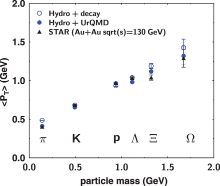
Mean P_T as a function of mass. The open circle symbols stand for hydro + decay, solid circle symbols stand for hydro + UrQMD, and solid triangle symbols stand for STAR data (Au+Au |$\sqrt {s_{NN}}=130$| GeV).

Open in new tabDownload slide

Let us now investigate the effect of resonance decays and hadronic rescattering on the pion and baryon transverse momentum spectra. Figure 16 shows the P_T spectrum of π⁺ at T_sw=150 MeV (solid line, uncorrected for resonance decays) as well as the final spectrum after hadronic rescattering and resonance decays, labeled as Hydro+UrQMD (solid symbols). In addition, the open symbols denote a calculation with the resonance decay correction performed at T_sw, which we label as Hydro+decay. The difference between the solid line and open symbols therefore directly quantifies the effect of resonance decays on the spectrum, which is most dominant in the low transverse momentum region P_T<1 GeV. Furthermore, the comparison between the open symbols and solid symbols quantifies the effect of hadronic rescattering: pions with P_T>1 GeV lose momenta via these final state interactions, resulting in the steeper slope.

Fig. 16.

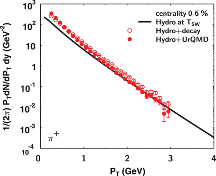
P_T spectra of π⁺ from hydro at the switching temperature (solid line), hydro+decay (open symbols), and hydro + UrQMD (solid symbols) in central collisions.

Open in new tabDownload slide

Figure 17 shows the elliptic flow as a function of η: the pure hydrodynamical calculation is shown by the solid curve, the hydrodynamical contribution at T_sw is denoted by the dashed line, and the full hydro+micro calculation is given by the solid circles, together with PHOBOS data (solid triangles). The shape of the elliptic flow in the pure hydrodynamical calculation at T_sw is quite different from that of the full hydrodynamical one terminated at the kinetic freezeout temperature, 110 MeV. Apparently the slight bumps at forward and backward rapidities observed in the full hydrodynamical calculation develop in the later hadronic phase, since they are not observed in the calculation terminated at T_sw. Evolving the hadronic phase in the hydro+micro approach increases the elliptic flow at the central rapidities, but not in the projectile and target rapidity regions. As a result, the result for the elliptic flow in the hydro+micro approach is closer to the experimental data compared to the pure hydrodynamical calculation.

Fig. 17.

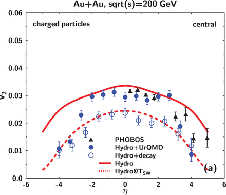
Elliptic flow as a function of η for π⁺ at centralities 5–10% and 10–20%. The open symbols stand for PHOBOS data and the solid symbols stand for our results.

Open in new tabDownload slide

In Fig. 18 we investigate the effect of hadronic rescattering on the duration of the freezeout process by comparing the calculation terminated at T_sw without hadronic rescattering (open symbols) and that including the full hadronic final state interactions (solid symbols). If we terminate time evolution at T_sw, most hadrons freeze out around τ_f=10 fm/c, reflecting the lifetime of the deconfined phase (the tails of the distribution come from the decays of long-lived resonances). The inclusion of hadronic rescattering shifts the peak of the freezeout distribution to larger freezeout times (τ_f∼20 to 30 fm), which provides an estimate of the lifetime of the hadronic phase around 10–20 fm.

Fig. 18.

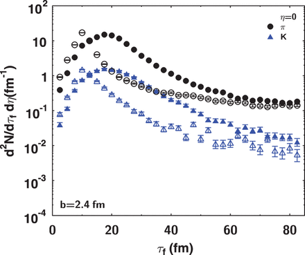
Freezeout time distribution of mesons for hydro+decay (open symbols) and hydro + UrQMD (solid symbols) at mid-rapidity in the case of central (0–5%) Au+Au collisions at top energy.

Open in new tabDownload slide

The findings discussed in the context of the previous figure for pions and kaons are confirmed by analyzing baryons in the same way, which is shown in Fig. 19: here, the top frame contains the analysis terminated at T_sw and the bottom frame contains the calculation including full hadronic rescattering. Figures 18 and 19 suggest that the assumption of sudden freezeout, which is often used in e.g. the blast wave model, is not realistic under the existence of final state interactions.

Fig. 19.

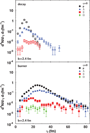
Freezeout time distribution of baryons for hydro+decay (open symbols, above) and hydro + UrQMD (solid symbols, below) at mid-rapidity in the case of central (0–5%) Au+Au collisions at top energy.

Open in new tabDownload slide

7. Summary

In this article, we have outlined key issues in constructing a realistic and comprehensive dynamical model for the description of all the stages of relativistic high energy heavy ion collisions: initial conditions, hydrodynamical expansion, hadronization, and freezeout processes. Hydrodynamical models are a promising starting point for building multi-module models. One of the reasons is that they give global understanding of experimental data at RHIC; their success at RHIC leads us to expect that hydrodynamical analyses will also serve as the baseline for investigations at LHC. In addition, one can easily input up-to-date knowledge on each stage in the time evolution to hydrodynamical models: more realistic initial conditions that contain event-by-event fluctuations, the latest equations of state and transport coefficients from lattice QCD, realistic hadronization mechanisms such as those from the recombination model and fragmentation mechanism, and realistic freezeout processes including final state interactions.

Currently, both ideal and viscous hydrodynamical models are utilized for the investigation of data obtained at RHIC and LHC. In multi-module modeling, however, ideal hydrodynamical models have been studied more deeply and they are considered to be more mature than viscous hydrodynamical models. However, gradually, the majority of hydrodynamical models will become viscous hydrodynamical models instead of ideal hydrodynamical models, because the study of viscosity effects in physical observables and the estimate of the viscosities in QGP from hadronic observables are among the hottest topics in the field; inclusion of viscosities in hydrodynamics is inevitable for such investigations. At the moment, investigations with viscous hydrodynamical models have just started. While their development has been fast and remarkable, a lot of issues remain to be considered, implemented, tested, and improved.

One of these issues is a numerical scheme for solving the relativistic hydrodynamical equation, to which only a little attention has so far been paid. In particular, the estimate of numerical viscosity is crucial for the study of the viscosities of the matter created in relativistic heavy ion collisions. In Sect. 4, we showed that the SHASTA, KT, and rHLLE schemes, which are mainly used in studies of high energy heavy ion collisions, have nearly the same accuracy and numerical artifacts. Furthermore, we showed the results of shock tube testing with a new numerical scheme that suffers a smaller artificial dissipative effect and showed that it is more suitable for analyses of physical viscosities than the SHASTA, KT, and rHLLE schemes.

In summary, in this article we have discussed in detail the essential ingredients in understanding entire stages of high energy heavy ion collisions, together with interpretation of experimental data at SPS, RHIC, and LHC. We hope that the road map shown in this article will serve as a guideline for modeling a realistic dynamical model for high energy heavy ion collisions.

Acknowledgements

We would like to thank Harry Niemi for providing us with the results shown in Figs. 9 and 10. This work was supported in part by a Grant-in-Aid for Young Scientists (B) (22740156) and Grants-in-Aid for Scientific Research (S) (22224003) and (C) (23540307).

References