 https://orcid.org/0000-0002-1458-8787
ABSTRACT
Radiative transfer modelling offers a powerful tool for understanding the enigmatic hydrogen emission lines from T Tauri stars. This work compares optical and near-IR spectroscopy of 29 T Tauri stars with our grid of synthetic line profiles. The archival spectra, obtained with VLT/X-Shooter, provide simultaneous coverage of many optical and infrared hydrogen lines. The observations exhibit similar morphologies of line profiles seen in other studies. We used the radiative transfer code torus to create synthetic H α, Pa β, Pa γ, and Br γ emission lines for a fiducial T Tauri model that included axisymmetric magnetospheric accretion and a polar stellar wind. The distribution of Reipurth types and line widths for the synthetic H α lines is similar to the observed results. However, the modelled infrared lines are narrower than the observations by |${\approx}80\,{~\rm km\,s}^{-1}$|, and our models predict a significantly higher proportion (≈90 per cent) of inverse P-Cygni profiles. Furthermore, our radiative transfer models suggest that the frequency of P-Cygni profiles depends on the ratio of the mass-loss to mass accretion rates and blue-shifted sub-continuum absorption was predicted for mass-loss rates as low as 10−12 M⊙ yr−1. We explore the effect of rotation, turbulence, and the contributions from red-shifted absorption in an attempt to explain the discrepancy in widths. Our findings show that, singularly, none of these effects is sufficient to explain the observed disparity. However, a combination of rotation, turbulence, and non-axisymmetric accretion may improve the fit of the models to the observed data.
1 INTRODUCTION
The progenitors of Sun-like stars are the T Tauri stars. They are low mass ≲2 M⊙, young pre-main-sequence stars known for their variability, strong magnetic fields, accretion disc, and mass outflows (Johns-Krull 2007; Hartmann, Herczeg & Calvet 2016). Classical T Tauri stars (CTTS) have observed excess ultraviolet (UV) and infrared continuum; their emission lines can be strong and have complex kinematic profiles (Reipurth, Pedrosa & Lago 1996). However, the origin of the radiation is not fully understood. By modelling the T Tauri emission, insight can be gained into the accretion, outflow, and the processes of angular momentum transfer present in these stars.
Koenigl (1991) proposed that the accretion mechanism is similar to that of neutron stars developed by Ghosh, Lamb & Pethick (1977). In this formalism, known as magnetospheric accretion, the magnetic field truncates the disc at a radius RT, where the magnetic and material stresses are of the same order. The accreting material free-falls from the disc to the stellar surface along the magnetic field, creating an accretion column or funnel. The in-falling matter thermalizes the kinetic energy as it impacts the stellar surface forming a shock zone or ‘hotspots’. The large energy release heats the gas to ≈106 K and could be responsible for the high blue and UV excesses observed from T Tauri stars (Hartmann et al. 2016). The presence of an extended magnetosphere allows for angular momentum transport, which may help explain the observed slow T Tauri rotation (Bouvier et al. 2014). Furthermore, the magnetospheric accretion can explain the red-shifted sub-continuum absorption, known as inverse P-Cygni (IPC) profiles, seen (e.g. Reipurth et al. (e.g. Edwards et al. 1994; Reipurth et al. 1996; Folha & Emerson 2001) in some T Tauri spectra.
Complex radiative transfer models were first employed to study magnetospheric accretion in T Tauri stars by Hartmann et al. (1994). They used a two-level hydrogen model to show that magnetospheric accretion could explain the strong emission lines and blue excess of several T Tauri stars. Muzerolle, Calvet & Hartmann (1998) further built on the T Tauri model by using a 2D radiative transfer code that performed a multilevel statistical equilibrium calculation for eight hydrogen levels. They concluded that the Br γ line profiles could be reproduced for embedded objects, and the Balmer line flux agreed with observations. Muzerolle et al. (1998) and Muzerolle, Calvet & Hartmann (2001) constrained the accretion column temperature to be between 6000 and 10 000 K and determined that Stark broadening may contribute to the observed broad H α wings (±500 km s−1). Bouvier et al. (2007) firmly established funnel-flow magnetospheric accretion paradigm, and it is now the generally accepted model for accretion in CTTS.
Blue-shifted sub-continuum absorption (the classical P-Cygni profile) is also observed and interpreted as evidence of the presence of mass outflow (e.g. Edwards et al. 2006; Kwan, Edwards & Fischer 2006). Kurosawa, Harries & Symington (2006) introduced a disc wind and polar stellar winds into their T Tauri radiative transfer simulations and were able to produce all seven classical line profile classes defined by Reipurth et al. (1996) for H α. Kurosawa, Romanova & Harries (2011) showed that a bipolar stellar wind could produce a broad P-Cygni absorption, whereas a narrow P-Cygni absorption was the product of a slow disc wind. Although it is not clear in which physical paradigms these outflow mechanisms are dominant or whether they coexist.
Another consideration for magnetospheric accretion is that the magnetic fields of T Tauri stars are rarely aligned with their poles (e.g. McGinnis, Bouvier & Gallet 2020). A magnetic obliquity will cause the accretion funnel to favour specific longitudes of the ascending nodes preferentially (Espaillat et al. 2021). A non-axisymmetric accretion funnel is likely to reduce the frequency of the observed IPC profiles, an effect that has been explored in several studies. For instance, Alencar et al. (2012) successfully used a non-axisymmetric accretion model, based on a magnetohydrodynamic (MHD) simulation, to perform a radiative transfer simulation of V2129 Oph* in H α and H β. However, they were unable to reproduce the red-shifted absorption accurately.
Despite the relative success of radiative transfer studies, the T Tauri models still have multiple free parameters and chronic degeneracy. It is unclear how to disentangle the effects of geometry, accretion, and mass-loss on the observed spectra. Consequently, although evidence supports the magnetospheric paradigm, the radiative transfer models need development before they can be comprehensively used as a diagnostic tool for T Tauri spectra. For example, Folha & Emerson (2001) noted that the current radiative transfer magnetospheric accretion models produced infrared lines (Paschen and Brackett) that were narrower than their observations by ≈100 km s−1.
The focus of this work is to present an initial comparison of synthetic and observed hydrogen line profiles, using the radiative transfer code torus (Harries et al. 2019). Our primary focus is on the model development and morphology of the synthetic spectra. This paper is structured as follows: initially, we introduce the T Tauri observations and data reduction in Section 2. We then describe in Section 3 the T Tauri model and the radiative transfer method. This section also outlines the parameters for our grid of synthetic hydrogen line profiles. The results of our parameter study, the comparison of the observations with the ensemble of synthetic profiles, and possible model modifications are presented in Section 4. Finally, we discuss the results and their implications in Section 5 and conclude in Section 6.
2 OBSERVATIONS AND DATA REDUCTION
We selected 29 T Tauri stars from the ESO programme 084.C-1095(A) observed on 2010 January 18, 19, and 20 (PI G. Herczeg; see Liu et al. 2016; Manara et al. 2016; Rugel et al. 2018; Schneider et al. 2018). The observed targets were selected to have a broad range of accretion rates of four orders of magnitude, the full list can be seen in Table 1. The observations were made using VLT’s X-Shooter instrument (Vernet et al. 2011) providing medium-resolution (R 11 600–18 400) spectra. The spectral range is 300–2480 nm divided into three parts, UVB, VIS, and NIR corresponding to the three independent cross-dispersed echelle spectrographs on X-Shooter, which are observed simultaneously. The spectra were obtained by nodding the telescope parallel to the slit. A slit width of 0.4 arcsec was used for all stars apart from DG Tau, which used a width of 1.2 arcsec. The spectra were flux calibrated during their initial reduction using the spectrophotometric standard star GD-71 (Manara et al. 2016).
The 29 T Tauri stars used in this work. Here, the notes ‘B’ or ‘T’ denote that the star is listed in the literature as a binary or triple system, respectively, a value of the angular separation is also given where available. The complete SIMBAD name for Stars named T-# are Ass-Cha-T-2-#. The masses, accretion rates, and notes are adopted from: (1) Manara et al. (2016), (2) Schneider et al. (2018), (3) Manara et al. (2014), (4) McGinnis et al. (2015), and (5) Rugel, Fedele & Herczeg (2018).
| Name | Type | Teff | AV | Mass | |$\log \dot{M}$| | Notes | Ref. |
|---|---|---|---|---|---|---|---|
| [K] | [mag] | [M⊙] | [M⊙ yr−1] | ||||
| ESO-Ha-562 | M0.5 + M0.5 | 3705 | 3.4 | 0.66 | −9.3 | B 0.28 arcsec | 1 |
| IQ-Tau | M0.5 | 3850 | 1.7 | 0.99 | −8.2 | 1 | |
| V354-Mon | K4 | 4900 | ∼ | 1.4 | −8 | 2 | |
| T-33 | K0 | 5110 | 2.7 | 0.95 | −8.7 | T 2.4 arcsec | 1 |
| T-11 | K2 | 4900 | 0.8 | 1.32 | 8.3 | B | 3 |
| VW-Cha | K7 + M0 | 4060 | 1.9 | 1.24 | −7.9 | B 0.66 arcsec | 1 |
| T-6 | K5 | 4350 | 0.51 | 1.22 | −7.8 | 3 | |
| CR-Cha | K0 | 5110 | 1.3 | 1.78 | −8.7 | 1 | |
| T-52 | K0 | 5110 | 1.0 | 1.4 | −7.4 | B 11.6 arcsec | 1 |
| T-38 | M0.5 | 3780 | 1.9 | 0.71 | −9.4 | 1 | |
| KV-Mon | K4 | ∼ | ∼ | 1.31 | ∼ | 4 | |
| Sz-22 | K5 | 4350 | 3.2 | 1.09 | −8.4 | T 17.6 arcsec | 1 |
| T-4 | K7 | 4060 | 0.5 | 1.03 | −9.5 | 1 | |
| DG-Tau | K5 | 4350 | 2.2 | 1.4 | −7.7 | 1 | |
| T-23 | M4.5 | 3200 | 1.7 | 0.33 | −8.3 | 1 | |
| RECX-12 | M3 | 3410 | ∼ | 0.29 | −9.8 | 5 | |
| Cha-Ha-6 | M6.5 | 2935 | 0.1 | 0.1 | −10.3 | 1 | |
| T-12 | M4.5 | 3200 | 0.8 | 0.23 | −8.8 | 1 | |
| CT-Cha-A | K5. | 4350 | 2.4 | 1.4 | −6.9 | 1 | |
| ESO-HA 442 | M2 | ∼ | ∼ | 0.36 | ∼ | 4 | |
| CHX18N | K2 | 4900 | 0.8 | 1.17 | −8.1 | 1 | |
| TW-Cha | K7. | 4060 | 0.8 | 1 | −9 | B | 1 |
| RECX-6 | M3 | 3415 | ∼ | 0.15 | −11 | 5 | |
| T-49 | M3.5 | 3340 | 1.0 | 0.36 | −7.6 | B 24.4 arcsec | 1 |
| T-35 | K7 | 4060 | 2.9 | 0.96 | −8.9 | 3 | |
| T-45a | K7 | 4060 | 1.1 | 0.97 | −9.9 | B 28.3 arcsec | 1 |
| RECX-9 | M4.5 | 3085 | ∼ | 0.15 | −10.4 | 5 | |
| T-24 | M0 | 3850 | 1.5 | 0.91 | −8.7 | 1 | |
| Hn-5 | M5 | 3125 | 0.0 | 0.16 | −9.3 | 1 |
| Name | Type | Teff | AV | Mass | |$\log \dot{M}$| | Notes | Ref. |
|---|---|---|---|---|---|---|---|
| [K] | [mag] | [M⊙] | [M⊙ yr−1] | ||||
| ESO-Ha-562 | M0.5 + M0.5 | 3705 | 3.4 | 0.66 | −9.3 | B 0.28 arcsec | 1 |
| IQ-Tau | M0.5 | 3850 | 1.7 | 0.99 | −8.2 | 1 | |
| V354-Mon | K4 | 4900 | ∼ | 1.4 | −8 | 2 | |
| T-33 | K0 | 5110 | 2.7 | 0.95 | −8.7 | T 2.4 arcsec | 1 |
| T-11 | K2 | 4900 | 0.8 | 1.32 | 8.3 | B | 3 |
| VW-Cha | K7 + M0 | 4060 | 1.9 | 1.24 | −7.9 | B 0.66 arcsec | 1 |
| T-6 | K5 | 4350 | 0.51 | 1.22 | −7.8 | 3 | |
| CR-Cha | K0 | 5110 | 1.3 | 1.78 | −8.7 | 1 | |
| T-52 | K0 | 5110 | 1.0 | 1.4 | −7.4 | B 11.6 arcsec | 1 |
| T-38 | M0.5 | 3780 | 1.9 | 0.71 | −9.4 | 1 | |
| KV-Mon | K4 | ∼ | ∼ | 1.31 | ∼ | 4 | |
| Sz-22 | K5 | 4350 | 3.2 | 1.09 | −8.4 | T 17.6 arcsec | 1 |
| T-4 | K7 | 4060 | 0.5 | 1.03 | −9.5 | 1 | |
| DG-Tau | K5 | 4350 | 2.2 | 1.4 | −7.7 | 1 | |
| T-23 | M4.5 | 3200 | 1.7 | 0.33 | −8.3 | 1 | |
| RECX-12 | M3 | 3410 | ∼ | 0.29 | −9.8 | 5 | |
| Cha-Ha-6 | M6.5 | 2935 | 0.1 | 0.1 | −10.3 | 1 | |
| T-12 | M4.5 | 3200 | 0.8 | 0.23 | −8.8 | 1 | |
| CT-Cha-A | K5. | 4350 | 2.4 | 1.4 | −6.9 | 1 | |
| ESO-HA 442 | M2 | ∼ | ∼ | 0.36 | ∼ | 4 | |
| CHX18N | K2 | 4900 | 0.8 | 1.17 | −8.1 | 1 | |
| TW-Cha | K7. | 4060 | 0.8 | 1 | −9 | B | 1 |
| RECX-6 | M3 | 3415 | ∼ | 0.15 | −11 | 5 | |
| T-49 | M3.5 | 3340 | 1.0 | 0.36 | −7.6 | B 24.4 arcsec | 1 |
| T-35 | K7 | 4060 | 2.9 | 0.96 | −8.9 | 3 | |
| T-45a | K7 | 4060 | 1.1 | 0.97 | −9.9 | B 28.3 arcsec | 1 |
| RECX-9 | M4.5 | 3085 | ∼ | 0.15 | −10.4 | 5 | |
| T-24 | M0 | 3850 | 1.5 | 0.91 | −8.7 | 1 | |
| Hn-5 | M5 | 3125 | 0.0 | 0.16 | −9.3 | 1 |
Note. ESO-HA 442 is also known as CID-0223980048.
The 29 T Tauri stars used in this work. Here, the notes ‘B’ or ‘T’ denote that the star is listed in the literature as a binary or triple system, respectively, a value of the angular separation is also given where available. The complete SIMBAD name for Stars named T-# are Ass-Cha-T-2-#. The masses, accretion rates, and notes are adopted from: (1) Manara et al. (2016), (2) Schneider et al. (2018), (3) Manara et al. (2014), (4) McGinnis et al. (2015), and (5) Rugel, Fedele & Herczeg (2018).
| Name | Type | Teff | AV | Mass | |$\log \dot{M}$| | Notes | Ref. |
|---|---|---|---|---|---|---|---|
| [K] | [mag] | [M⊙] | [M⊙ yr−1] | ||||
| ESO-Ha-562 | M0.5 + M0.5 | 3705 | 3.4 | 0.66 | −9.3 | B 0.28 arcsec | 1 |
| IQ-Tau | M0.5 | 3850 | 1.7 | 0.99 | −8.2 | 1 | |
| V354-Mon | K4 | 4900 | ∼ | 1.4 | −8 | 2 | |
| T-33 | K0 | 5110 | 2.7 | 0.95 | −8.7 | T 2.4 arcsec | 1 |
| T-11 | K2 | 4900 | 0.8 | 1.32 | 8.3 | B | 3 |
| VW-Cha | K7 + M0 | 4060 | 1.9 | 1.24 | −7.9 | B 0.66 arcsec | 1 |
| T-6 | K5 | 4350 | 0.51 | 1.22 | −7.8 | 3 | |
| CR-Cha | K0 | 5110 | 1.3 | 1.78 | −8.7 | 1 | |
| T-52 | K0 | 5110 | 1.0 | 1.4 | −7.4 | B 11.6 arcsec | 1 |
| T-38 | M0.5 | 3780 | 1.9 | 0.71 | −9.4 | 1 | |
| KV-Mon | K4 | ∼ | ∼ | 1.31 | ∼ | 4 | |
| Sz-22 | K5 | 4350 | 3.2 | 1.09 | −8.4 | T 17.6 arcsec | 1 |
| T-4 | K7 | 4060 | 0.5 | 1.03 | −9.5 | 1 | |
| DG-Tau | K5 | 4350 | 2.2 | 1.4 | −7.7 | 1 | |
| T-23 | M4.5 | 3200 | 1.7 | 0.33 | −8.3 | 1 | |
| RECX-12 | M3 | 3410 | ∼ | 0.29 | −9.8 | 5 | |
| Cha-Ha-6 | M6.5 | 2935 | 0.1 | 0.1 | −10.3 | 1 | |
| T-12 | M4.5 | 3200 | 0.8 | 0.23 | −8.8 | 1 | |
| CT-Cha-A | K5. | 4350 | 2.4 | 1.4 | −6.9 | 1 | |
| ESO-HA 442 | M2 | ∼ | ∼ | 0.36 | ∼ | 4 | |
| CHX18N | K2 | 4900 | 0.8 | 1.17 | −8.1 | 1 | |
| TW-Cha | K7. | 4060 | 0.8 | 1 | −9 | B | 1 |
| RECX-6 | M3 | 3415 | ∼ | 0.15 | −11 | 5 | |
| T-49 | M3.5 | 3340 | 1.0 | 0.36 | −7.6 | B 24.4 arcsec | 1 |
| T-35 | K7 | 4060 | 2.9 | 0.96 | −8.9 | 3 | |
| T-45a | K7 | 4060 | 1.1 | 0.97 | −9.9 | B 28.3 arcsec | 1 |
| RECX-9 | M4.5 | 3085 | ∼ | 0.15 | −10.4 | 5 | |
| T-24 | M0 | 3850 | 1.5 | 0.91 | −8.7 | 1 | |
| Hn-5 | M5 | 3125 | 0.0 | 0.16 | −9.3 | 1 |
| Name | Type | Teff | AV | Mass | |$\log \dot{M}$| | Notes | Ref. |
|---|---|---|---|---|---|---|---|
| [K] | [mag] | [M⊙] | [M⊙ yr−1] | ||||
| ESO-Ha-562 | M0.5 + M0.5 | 3705 | 3.4 | 0.66 | −9.3 | B 0.28 arcsec | 1 |
| IQ-Tau | M0.5 | 3850 | 1.7 | 0.99 | −8.2 | 1 | |
| V354-Mon | K4 | 4900 | ∼ | 1.4 | −8 | 2 | |
| T-33 | K0 | 5110 | 2.7 | 0.95 | −8.7 | T 2.4 arcsec | 1 |
| T-11 | K2 | 4900 | 0.8 | 1.32 | 8.3 | B | 3 |
| VW-Cha | K7 + M0 | 4060 | 1.9 | 1.24 | −7.9 | B 0.66 arcsec | 1 |
| T-6 | K5 | 4350 | 0.51 | 1.22 | −7.8 | 3 | |
| CR-Cha | K0 | 5110 | 1.3 | 1.78 | −8.7 | 1 | |
| T-52 | K0 | 5110 | 1.0 | 1.4 | −7.4 | B 11.6 arcsec | 1 |
| T-38 | M0.5 | 3780 | 1.9 | 0.71 | −9.4 | 1 | |
| KV-Mon | K4 | ∼ | ∼ | 1.31 | ∼ | 4 | |
| Sz-22 | K5 | 4350 | 3.2 | 1.09 | −8.4 | T 17.6 arcsec | 1 |
| T-4 | K7 | 4060 | 0.5 | 1.03 | −9.5 | 1 | |
| DG-Tau | K5 | 4350 | 2.2 | 1.4 | −7.7 | 1 | |
| T-23 | M4.5 | 3200 | 1.7 | 0.33 | −8.3 | 1 | |
| RECX-12 | M3 | 3410 | ∼ | 0.29 | −9.8 | 5 | |
| Cha-Ha-6 | M6.5 | 2935 | 0.1 | 0.1 | −10.3 | 1 | |
| T-12 | M4.5 | 3200 | 0.8 | 0.23 | −8.8 | 1 | |
| CT-Cha-A | K5. | 4350 | 2.4 | 1.4 | −6.9 | 1 | |
| ESO-HA 442 | M2 | ∼ | ∼ | 0.36 | ∼ | 4 | |
| CHX18N | K2 | 4900 | 0.8 | 1.17 | −8.1 | 1 | |
| TW-Cha | K7. | 4060 | 0.8 | 1 | −9 | B | 1 |
| RECX-6 | M3 | 3415 | ∼ | 0.15 | −11 | 5 | |
| T-49 | M3.5 | 3340 | 1.0 | 0.36 | −7.6 | B 24.4 arcsec | 1 |
| T-35 | K7 | 4060 | 2.9 | 0.96 | −8.9 | 3 | |
| T-45a | K7 | 4060 | 1.1 | 0.97 | −9.9 | B 28.3 arcsec | 1 |
| RECX-9 | M4.5 | 3085 | ∼ | 0.15 | −10.4 | 5 | |
| T-24 | M0 | 3850 | 1.5 | 0.91 | −8.7 | 1 | |
| Hn-5 | M5 | 3125 | 0.0 | 0.16 | −9.3 | 1 |
Note. ESO-HA 442 is also known as CID-0223980048.
Telluric corrections were applied using ESO’s Molecfit pipeline (Smette et al. 2015; Kausch et al. 2015). The hydrogen lines H α (2-3, 6562 Å), Pa β (3-5, 12818 Å), Pa γ (3-6, 10938 Å) and Br γ (4-7, 21655 Å) were extracted from the full X-Shooter spectra. The profiles were normalized by fitting a third-order polynomial to the nearby continuum. Veiling is expected to influence the equivalent widths of the optical and infrared lines due to excess emission from the accretion and warm dust in the disc. Although the profiles are presented in continuum normalized space, the ISM extinction will influence the unnormalized fluxes. The star’s Cardelli, Clayton & Mathis (1989) extinction law reddening corrections are given in Table 1. However, the effects of veiling and extinction are not addressed in this work and are left to a future paper. Instead, the focus is on the line morphology and width, characteristics independent of the veiling and extinction.
The hydrogen line profiles from X-Shooter can be seen in Fig. 1. The figure shows the continuum normalized line profiles for the target stars arranged in order of H α intensity. Each column displays the spectra for the individual objects listed in Table 1 at four different wavelengths, centred on H α, Pa γ, Pa β, and Br γ. Some stars with strong H α emission, e.g. Cha Ha 6, CID 0223980048 (ESO-HA 442), and Ass Cha T 2-33 have undetected emission in the Paschen and Brackett lines.
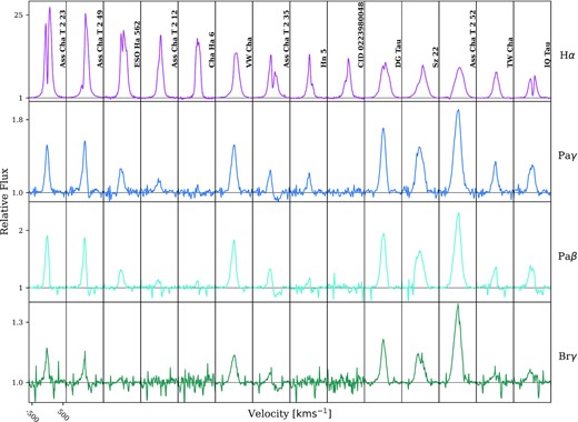

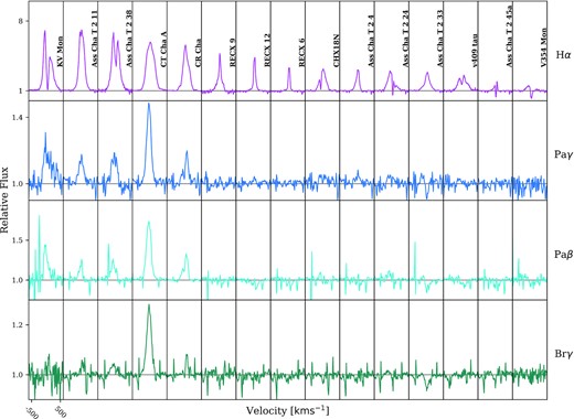
The normalized X-Shooter spectra of the objects (columns) listed in Table.1, at four different wavelengths: H α; 6562 Å, Pa γ; 10 938 Å, Pa β; 12 818 Å, and Br γ; 21 655 Å. The relative flux is plotted as a function of velocity, and each column has a width of ±500 km s−1. The stars are arranged left to right by H α peak intensity.
Following the scheme set out by Reipurth et al. (1996), the emission-line profiles were classified as follows.
Type I: symmetric profiles with little or no features.
Type II: two peaks, the second being greater than half the strength of the primary.
Type III: two peaks, the second being less than half the strength of the primary.
Type IV: sub-continuum absorption with no further significant emission beyond the absorption.
The types are subdivided into B or R, depending on if the absorption feature is blue-shifted or red-shifted relative to the primary peak. Types IVB and IVR are analogous to P-Cygni and IPC profiles, respectively.
Fig. 2 shows the Reipurth classification for the observations and the synthetic profiles. The latter are discussed in Section 4. The line profiles were classified by eye. The seven types of profile morphology defined by Reipurth et al. (1996) are seen in the data. For spectra where the Reipurth type was not easily determined due to the noise levels, the profiles were not classified and excluded from the results of this paper. Therefore, these unclassified spectra introduce an uncertainty into the Reipurth distribution. The number of unclassified spectra are: 0 H α, 10 Pa β, 14 Pa γ, and 18 Br γ. The sample of T Tauri stars is comparatively small and a significant proportion of the infrared lines could not be classified. Consequently, the statistical significance of the distribution is ambiguous; however, it exhibits a similar distribution of morphologies as those seen in previous T Tauri studies (e.g. Folha & Emerson 2001; Reipurth et al. 1996). The distribution concurs with the previous results in showing that the majority (≈43 per cent) of profiles are type I and the second highest population of Reipurth types for the infrared lines are type IVR.
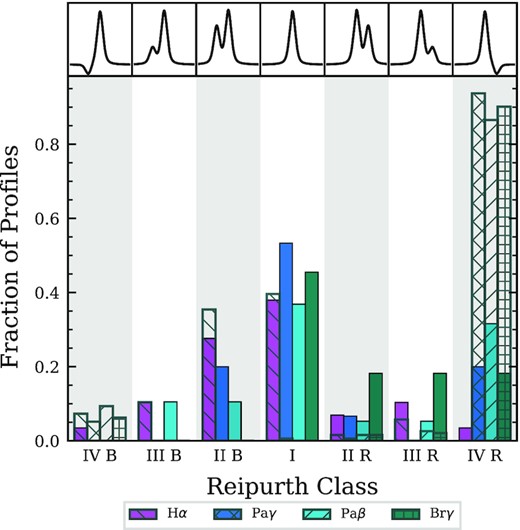
Relative percentage of Reipurth classification. The coloured bars indicate the results for the X-Shooter observations. The results are subdivided by hydrogen emission line and an example profile of each type is shown at the top. The hashed bars overplotted are the classification of the corresponding synthetic emission lines.

There are several cases of IPC profiles in our data, the majority of which are seen for Pa β. There are two notable stars that contain prominent IPC signatures across all the infrared lines. Ass Cha T 2-35 has strong IPC absorption in all the infrared lines. Whereas, the H α line only displays a red-shifted secondary peak. Ass Cha T 2-49 has a narrow IPC absorption in the infrared lines and no significant H α red-shifted absorption. Blue-shifted absorption is even more rare in our data. For instance, Ass Cha T 2-52 has a narrow H α P-Cygni absorption profile consistent with a disc wind (Kurosawa et al. 2011). None of the infrared lines exhibit discernible blue-shifted absorption.
Four of the observed stars are classified as weak line T Tauri stars, according to the classification scheme of White & Basri (2003), because their half widths at 10 per cent maximum (HW10 per cent) are less than 135 km s−1. The stars are RECX-6, Ass Cha T 2-45a, Ass Cha T 2-4, and RECX-12. In this work, we adopt the HW10 per cent criterion because White & Basri (2003) showed it to be a reliable method of distinguishing between classical and weak line T Tauri stars and the HW10 per cent criterion is unaffected by veiling.
3 RADIATIVE TRANSFER MODELLING
To create synthetic T Tauri hydrogen emission lines, we used the radiative transfer code torus (Harries et al. 2019). The code uses an analytical model as an input that approximates the expected geometry, density, temperature, velocity, emission, and absorption sources in a 3D space. These include the disc, star, magnetospheric accretion, and stellar wind. torus then uses this model to calculate the expected population levels and create synthetic spectra.
3.1 T Tauri accretion and outflow model
torus uses an adaptive mesh refinement (AMR) system to create a numerical grid representing the physical space of the simulation (see Fig. 3). The simulations presented in this work use a 2.5D model, and they are axisymmetric around the pole. The 2.5D geometry is defined using a 2D density field and a 3D velocity field. The third component is calculated symmetrically for a given azimuthal angle.
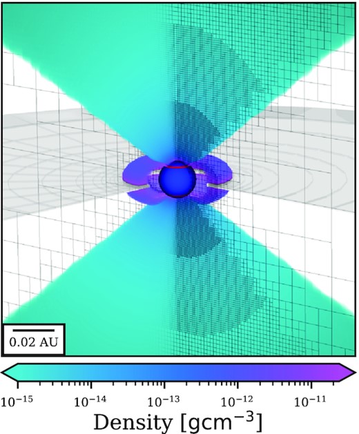
A 3D render of the T Tauri model from torus with a section of the stellar wind and accretion funnel cut away. The colour scale of the accretion funnel and stellar wind denote density. The hotspot is shown on the stellar surface as a red band. The adaptive mesh (grey lines) uses a higher frequency of cells for denser regions. The disc shown is a schematic to portray the position of the geometrically thin, optically thick disc.

The mesh is populated with volumes of space that are filled with a star, an accretion flow, and a stellar wind (see Fig. 4). An accretion disc is represented by an opaque, infinitely thin plane in the equatorial region of the grid, with a circular gap in the centre, containing the accretion flow and star. The density, temperature, and velocity fields are defined as outlined in Sections 3.1.1 and 3.1.2. The star, placed at the origin, is defined by its radius R*, mass M*, and effective temperature Teff. The stellar continuum is interpolated from tabulated Kurucz model atmospheres (Kurucz 1979).
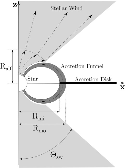
A cartoon depicting the T Tauri model geometry used in this paper. The models are axisymmetric around the Z-axis. The stellar wind becomes radial beyond Rwo, defined as the radius at which the magnetically connected wind expands to the prescribed opening angle Θsw. Not to scale.

The AMR grid starts with four cells and is subsequently refined algorithmically by splitting the cells into four subcells, such that the mass of each cell is <1010 g. Each cell can be subdivided a maximum of 10 times. The total size of the simulation space was set to be a 3D cylindrical mesh with a height and radius of 400 × 1010 cm. The minimum cell size therefore has a length of 0.39 × 1010 cm.
3.1.1 Accretion funnel
Model parameters.
| Parameter | Value | Unit | Description | |
|---|---|---|---|---|
| M* | 0.5 | M⊙ | Star mass | |
| Star | R* | 2.0 | R⊙ | Star radius |
| Teff | 4000 | K | Effective stellar temperature | |
| AccretionFunnel | Rmi | 2.2 | R* | Truncation radius and inner magnetosphere connection point |
| Rmo | 3.0 | R* | Outer connection point of magnetosphere | |
| Tacc | 6500, 7500, 8500, 9500 | K | Maximum temperature of magnetosphere | |
| |$\dot{M}_{\rm acc}$| | 10−7, 10−8, 10−9 | M⊙ yr−1 | Magnetospheric accretion rate | |
| Vrot | 0.0 | km s−1 | Rotation velocity | |
| Θsw | 50 | |$\deg$| | Stellar wind opening angle | |
| vmin | 10 | km s−1 | Velocity of wind at launch | |
| Stellar | vmax | 400 | km s−1 | Maximum wind velocity |
| Wind | β | 2.89 | Wind velocity scaling | |
| |$\dot{M}_{\rm sw}$| | 0.1,0.01,0.001 | |$\dot{M}_{\rm acc}$| | Mass-loss rate as a fraction of accretion rate | |
| Tsw | 6000,8000,10 000 | K | Isothermal wind temperature | |
| Synthetic | inc | 20,60,80 | deg | Co-latitude of synthetic profile viewing angle |
| Profile | λ | 6562, 10 938, 12 818, 21 655 | Å | Observed wavelengths: H α, Pa γ, Pa β, and Br γ, respectively |
| Parameter | Value | Unit | Description | |
|---|---|---|---|---|
| M* | 0.5 | M⊙ | Star mass | |
| Star | R* | 2.0 | R⊙ | Star radius |
| Teff | 4000 | K | Effective stellar temperature | |
| AccretionFunnel | Rmi | 2.2 | R* | Truncation radius and inner magnetosphere connection point |
| Rmo | 3.0 | R* | Outer connection point of magnetosphere | |
| Tacc | 6500, 7500, 8500, 9500 | K | Maximum temperature of magnetosphere | |
| |$\dot{M}_{\rm acc}$| | 10−7, 10−8, 10−9 | M⊙ yr−1 | Magnetospheric accretion rate | |
| Vrot | 0.0 | km s−1 | Rotation velocity | |
| Θsw | 50 | |$\deg$| | Stellar wind opening angle | |
| vmin | 10 | km s−1 | Velocity of wind at launch | |
| Stellar | vmax | 400 | km s−1 | Maximum wind velocity |
| Wind | β | 2.89 | Wind velocity scaling | |
| |$\dot{M}_{\rm sw}$| | 0.1,0.01,0.001 | |$\dot{M}_{\rm acc}$| | Mass-loss rate as a fraction of accretion rate | |
| Tsw | 6000,8000,10 000 | K | Isothermal wind temperature | |
| Synthetic | inc | 20,60,80 | deg | Co-latitude of synthetic profile viewing angle |
| Profile | λ | 6562, 10 938, 12 818, 21 655 | Å | Observed wavelengths: H α, Pa γ, Pa β, and Br γ, respectively |
Model parameters.
| Parameter | Value | Unit | Description | |
|---|---|---|---|---|
| M* | 0.5 | M⊙ | Star mass | |
| Star | R* | 2.0 | R⊙ | Star radius |
| Teff | 4000 | K | Effective stellar temperature | |
| AccretionFunnel | Rmi | 2.2 | R* | Truncation radius and inner magnetosphere connection point |
| Rmo | 3.0 | R* | Outer connection point of magnetosphere | |
| Tacc | 6500, 7500, 8500, 9500 | K | Maximum temperature of magnetosphere | |
| |$\dot{M}_{\rm acc}$| | 10−7, 10−8, 10−9 | M⊙ yr−1 | Magnetospheric accretion rate | |
| Vrot | 0.0 | km s−1 | Rotation velocity | |
| Θsw | 50 | |$\deg$| | Stellar wind opening angle | |
| vmin | 10 | km s−1 | Velocity of wind at launch | |
| Stellar | vmax | 400 | km s−1 | Maximum wind velocity |
| Wind | β | 2.89 | Wind velocity scaling | |
| |$\dot{M}_{\rm sw}$| | 0.1,0.01,0.001 | |$\dot{M}_{\rm acc}$| | Mass-loss rate as a fraction of accretion rate | |
| Tsw | 6000,8000,10 000 | K | Isothermal wind temperature | |
| Synthetic | inc | 20,60,80 | deg | Co-latitude of synthetic profile viewing angle |
| Profile | λ | 6562, 10 938, 12 818, 21 655 | Å | Observed wavelengths: H α, Pa γ, Pa β, and Br γ, respectively |
| Parameter | Value | Unit | Description | |
|---|---|---|---|---|
| M* | 0.5 | M⊙ | Star mass | |
| Star | R* | 2.0 | R⊙ | Star radius |
| Teff | 4000 | K | Effective stellar temperature | |
| AccretionFunnel | Rmi | 2.2 | R* | Truncation radius and inner magnetosphere connection point |
| Rmo | 3.0 | R* | Outer connection point of magnetosphere | |
| Tacc | 6500, 7500, 8500, 9500 | K | Maximum temperature of magnetosphere | |
| |$\dot{M}_{\rm acc}$| | 10−7, 10−8, 10−9 | M⊙ yr−1 | Magnetospheric accretion rate | |
| Vrot | 0.0 | km s−1 | Rotation velocity | |
| Θsw | 50 | |$\deg$| | Stellar wind opening angle | |
| vmin | 10 | km s−1 | Velocity of wind at launch | |
| Stellar | vmax | 400 | km s−1 | Maximum wind velocity |
| Wind | β | 2.89 | Wind velocity scaling | |
| |$\dot{M}_{\rm sw}$| | 0.1,0.01,0.001 | |$\dot{M}_{\rm acc}$| | Mass-loss rate as a fraction of accretion rate | |
| Tsw | 6000,8000,10 000 | K | Isothermal wind temperature | |
| Synthetic | inc | 20,60,80 | deg | Co-latitude of synthetic profile viewing angle |
| Profile | λ | 6562, 10 938, 12 818, 21 655 | Å | Observed wavelengths: H α, Pa γ, Pa β, and Br γ, respectively |
3.1.2 Stellar wind
We implemented a new stellar wind in torus that builds on the work by Kurosawa et al. (2011). Their model used a radial stellar wind launched from a spherical cap above the stellar surface so that a large opening angle could be achieved without interacting with the accretion funnel. The new wind geometry launches the outflow from the stellar surface from the polar region at higher latitudes than the accretion hotspot. The wind and accretion funnel do not intersect because the wind follows the dipole magnetic field lines until it reaches a specified opening angle Θsw, at which point the wind becomes radial (see Fig. 4). The parametrization of Θsw automatically determines the radius Rwo where the wind transitions from following the dipole lines to becoming radial. This geometry approximates the wind behaviour that is observed in MHD simulations (e.g. Zanni & Ferreira 2009; Kurosawa & Romanova 2012; Ireland et al. 2021). The wind is assumed to be isothermal.
3.2 Radiative transfer
To model the radiative emission of T Tauri stars, we use the radiative transfer code torus, which has previously been used to model the emission from T Tauri stars (e.g. Symington, Harries & Kurosawa 2005; Kurosawa et al. 2006, 2011). However, the treatment of the radiation field has significantly diverged from prior versions. torus now uses an atomic statistical equilibrium integration method based on the accelerated Monte Carlo scheme developed by Hogerheijde & van der Tak (2000), in which rays are propagated to random positions in a cell in random directions. The radiative transfer equation is solved along these rays to find the local continuum radiation field. This method accelerates the convergence of the simulation in areas of significant optical depth. Additionally, torus uses full-frame co-moving ray tracing to create synthetic hydrogen line profiles. torus computes the line profiles in two stages. First, it calculates the level populations assuming statistical equilibrium, and secondly, torus computes the line profiles using full-frame co-moving ray tracing. This method is known as Sobolev with exact integration (SEI; Harries et al. 2019).
3.2.1 Statistical equilibrium
3.2.2 Synthetic line profiles
Once the level populations have been calculated, torus can compute synthetic observations to model how the system will appear to the observer. The synthetic observations created in this work by torus are position–position−velocity (PPV) datacubes containing both spectral and spacial information. The synthetic line profiles are calculated using full-frame co-moving ray tracing, which allows for pressure broadening of the lines and is better suited to dealing with regions of high optical depth when scattering is not significant. For atomic statistical equilibrium, torus does not account for scattering and only the total intensity is considered. Pressure broadening is traditionally considered important because T Tauri Balmer lines can have wings that extend up to ±500 km s−1 (e.g. Edwards et al. 1994). These broad wings are hard to achieve with model geometry alone and may be the result of Stark broadening (Muzerolle et al. 1998, 2001).
Initially, each cell of the AMR mesh is divided into two ray segments, but this number is doubled if dτν > 0.1 and dτν < 20. Furthermore, if the velocity gradient across the cell would cause the line resonance to be traversed or ν is close to line resonance the number of segments is set to 20.
The Stark broadening has a significant impact on the H α line widths at high accretion rates and funnel flow temperatures, see Section 3.3. By using half-widths determined from the extended VCS tables (Lemke 1997), we found that for Pa γ, Pa β, and Br γ Stark broadening had a negligible effect.
By integrating the total surface brightness in each of the PPV datacube’s frames, the synthetic line profile of the flux versus velocity is calculated. The flux is normalized relative to the first velocity bin of the datacube, which is assumed to be the continuum. This is correct as long as the full extent of the line profile is covered by the wavelength range of the datacube and the initial frame does not have any line emission. The synthetic continuum includes emission from the stellar photosphere and accretion hotspot. The emission from dust is not included in these models. torus can run a Monte Carlo radiative transfer loop, along side the atomic statistical equilibrium calculation to determine the emission from dust; however, this is left to a future paper.
3.3 Model validation
A comparison of the results produced by Kurosawa et al. (2006) and torus can be seen in Fig. 5. We ran the model on torus using both linear and non-linear Stark broadening. Fig. 5 demonstrates that the new radiative transfer scheme produces results in satisfactory agreement with the models of Kurosawa et al. (2006). The H α lines produced using torus are slightly broader, with higher peak intensities than those presented by Kurosawa et al. (2006). There are only negligible differences between the lines computed with linear and non-linear Stark broadening.
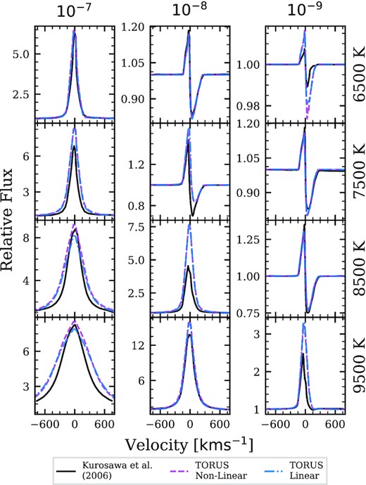
A comparison of synthetic H α line profiles produced by Kurosawa et al. (2006) (black lines) and torus. The models have magnetospheric accretion only and no form of mass outflows. Profiles arrange by accretion rate (columns) in values of M⊙yr−1 and accretion maximum temperature (rows) for a viewing colatitude of 55°. Two different Stark broadening parametrizations are used by torus; linear (blue dot–dashed) and non-linear (pink dashed) Stark broadening. Line strength increases with temperature and accretion rate, top-right to bottom-left.

The general line profile trends shown by Kurosawa et al. (2006) are reflected by our torus models. The line strength and width increase with the accretion temperature and rates. An exception to this trend is seen in Fig. 5 for the line profile produced with an accretion rate of |$\log {\dot{M}_{\rm acc}}=-8$| and Tacc = 9500 K. The line profile has a greater relative peak flux than the profile produced with an accretion rate of |$\log {\dot{M}_{\rm acc}}=-7$|. This is because the continuum level from the hotspot is increased by the greater accretion rate, reducing the peak flux relative to the continuum. We see, in Fig. 5, that the width of the profiles increases with the rate and temperature of the accretion; it is unaffected by the continuum level.
The above comparisons did not include any outflows. Therefore, to test our stellar wind geometry (Section 3.1.2) we ran an additional test to compare our model with the stellar wind geometry used by Kurosawa et al. (2011). These results are not shown but they are described below. torus was used to run two models with identical stellar and magnetospheric parameters as those defined for fig. 10 of Kurosawa et al. (2011). The first models had an identical wind as Kurosawa et al. (2011); the wind launched from 3R* above the star’s surface. The second model used our wind geometry with the outflow being launched from the star’s surface. We adopted the same outflow parameters of Tsw, |$\dot{M}_{\rm sw}$|, vmin, vmax, and Θopen. The second model also used a value of β = 1.6 rather than β = 0.5 as this more closely matched the wind acceleration and velocity at radii greater than 3R*.
The differences in the line profiles produced by the two wind models are modest, comparable in magnitude to the variations seen in Fig. 5. For H α at low colatitude, the lines produced by our stellar wind model were broader at the peak by ≈20 km s−1. For high colatitudes, the lines were slightly narrower and exhibited small-scale blue-shifted absorption features not seen in the Kurosawa et al. (2011) wind model. For the higher lines, at inclinations of 20° and 50°, the wind that extended to the star’s surface produced lines that were narrower and had a lower peak flux. Our wind model also produced deeper red-shifted absorption than the model of Kurosawa et al. (2011). These effects, however, are likely to not be discernible in T Tauri observations. Nevertheless, the new wind geometry was used in this work because it is more physically realistic.
3.4 Parameter study
We present a grid of synthetic models covering a broad range of temperatures and accretion rates, with the parameters shown in Table 2. The models have a single source star with an effective temperature of Teff = 4000 K, a mass of M* = 0.5 M⊙, and a radius of R* = 2.0 R⊙. Our grid covers a broad range of accretion rates of 10−7, 10−8, and 10−9 M⊙ yr−1 with mass-loss rates of 0.1, 0.01, and 0.001 of the accretion rate. These mass-loss rates were selected to be in the required range to provide a significant ‘spin-down’ torque on the star (Matt & Pudritz 2005) and are consistent with the range of values estimated from jets (Nisini et al. 2018). The source star parameters and the wind and magnetospheric geometries were not varied. For each model configuration, synthetic line profiles were computed for three inclinations (20°, 60°, 80°) centred on the four hydrogen emission lines of the observational data set described in Section 2.
Fig. 6 shows a subset of line profiles in the grid; only models with a mass-loss rate of |$0.01~\dot{M}_{\rm acc}$| and wind temperature of 8000 K are included. The figure arranges the line profiles by accretion rate and maximum magnetospheric temperature, subdivided by the hydrogen transition. The synthetic lines exhibit a broad range of different morphologies. H α has the highest peak intensity, and the subsequent strongest lines are Pa β, Pa γ, and Br γ, respectively. However, ≈7 per cent of the Br γ lines at an inclination of 20° have a greater peak intensity than Pa β and Pa γ. These lines occur for an accretion temperature of |$9500{~\rm K}$| and an accretion rate of |$10^{-7}{~\rm M}_{\odot }\,{\rm yr}^{-1}$|. The H α lines are in general broader than the infrared lines, with a few having broad wings >1000 km s−1. The majority (≈83 per cent) of the infrared lines display red-shifted absorption from the magnetosphere. Blue-shifted sub-continuum absorption is not seen at high inclination where the viewing angle is along the disc outside of the wind opening angle.
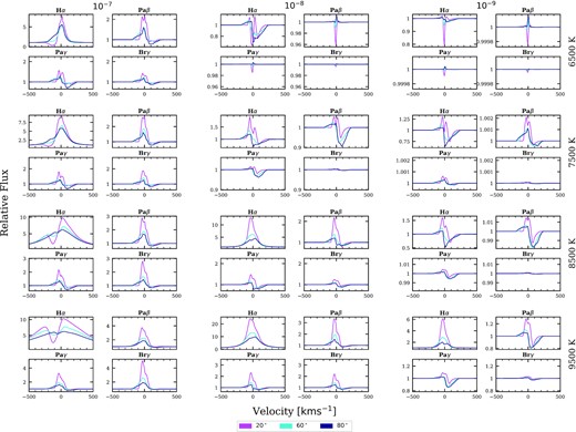
A sample of the line profiles produced by torus. The spectra are shown for |$\dot{M}_{\rm sw}=0.01~\dot{M}_{\rm acc}$| and Tsw = 8000 K. The lines are arranged by |$\dot{M}_{\rm acc}$| (columns) and Tacc (rows). Each section is subdivided by hydrogen transition and shows the three different inclinations (colours). The y-axes of Pa γ, Pa β, and Br γ for each set, share a common range. IPC profiles are present in the majority of the infrared lines. For the hydrogen transitions at an inclination of 80° (outside of the stellar wind opening angle), there is less blue-shifted absorption and no P-Cygni features. H α profiles are broad with some wings exceeding 500 km s−1.

4 RESULTS
The general trends seen in the grid of synthetic line profiles are outlined as follows. Higher accretion rates increase the line width and intensity. A high accretion rate of |$\log {\dot{M}_{\rm acc}}=-6$| produced structured H α absorption superposed on broad (±1000 km s−1) emission profiles. Only a limited number of models with an accretion rate of |$\log {\dot{M}_{\rm acc}}=-6$| were run and the profiles are not included in this paper. The line profile intensity increases with magnetospheric temperature. The H α lines are dominated by Stark broadening for accretion flow temperatures of at least 7500 K at accretion rates of |$\log {\dot{M}_{\rm acc}}\ge -8$|. The Stark broadening significantly increases the line widths and is highly dependent on the magnetospheric temperature and density. For a temperature of 9500 K and an accretion rate of |$\log {\dot{M}_{\rm acc}}=-7$|, the H α profiles are Stark broadened to have wings of over ±1000 km s−1. Conversely, the infrared lines are almost completely unaffected by Stark broadening. The intensity and equivalent width of the infrared lines increase significantly with greater accretion rates and temperature. Whereas, the full width at half-maximum (FWHM) of the profiles are less strongly affected by the rate and temperature of the accretion flow.
H α exhibits IPC profiles for accretion rates of |$\log {\dot{M_{\rm acc}}}=-8$| when |$T_{\rm acc} \le 7500{~\rm K}$| and for |$\log {\dot{M}_{\rm acc}}=-9$| when |$T_{\rm acc} \le 8500{~\rm K}$|. For accretion rates and temperatures above this, the Stark broadening smooths over the absorption features. For the infrared lines, the IPC profiles are exhibited irrespective of inclination, accretion rate, or temperature.
Strong P-Cygni profiles are seen when the wind outflow rate is |$\ge 0.01\dot{M}_{\rm acc}$| and the inclination is within the stellar wind opening angle. The continuum relative depth of the blue-shifted absorption increases with the wind temperature. The line intensity is inversely correlated with the wind temperatures. This is particularly apparent for the infrared lines, because the higher energy levels, 5, 6, and 7, become depopulated before the upper H α level. However, this inverse relationship does not hold at a high wind temperature (2 × 10⁴ K), where emission from the wind dominates when the mass-loss rate is |$\ge 0.01\dot{M}_{\rm acc}$|.
The frequency of P-Cygni profiles is correlated with the ratio |$\dot{M}_{\rm sw}/\dot{M}_{\rm acc}$| and not |$\dot{M}_{\rm sw}$| alone. For example, at a high accretion rate of |$\log {\dot{M}_{\rm acc}}=-7$|, P-Cygni profiles are only seen at mass-loss rates of |$\log {\dot{M}_{\rm sw}}=-8$| and −9. Whereas, for an accretion rate of |$\log {\dot{M}_{\rm acc}}=-8$|, P-Cygni profiles are seen for mass-loss rates of |$\log {\dot{M}_{\rm sw}}=-9$|, −10, and −11 with decreasing frequency. Similar results are seen for an accretion rate of |$\log {\dot{M}_{\rm acc}}=-9$|. P-Cygni profiles were produced for mass-loss rates as low as 10−12 M⊙ yr−1. At higher accretion rates, the emission from the magnetosphere more commonly dominates, overwhelming the blue-shifted absorption.
The synthetic line profiles were calculated for velocity increments of Δv = 12.04 km s−1, which corresponds to a spectral resolution of R = 24 900. The observations are observed at resolutions of R = 18 400 (16 km s−1) for H α and R = 11 600 (26 km s−1) for the infrared lines. We explored the effect of applying a Gaussian convolution to the synthetic spectra to reduce their resolution to the resolution of the observed spectra. However, the change in line profile morphology, in particular the FWHM and HW10 per cent, was negligible when the synthetic spectra were convolved. Therefore, convolution was not considered a significant factor and not included in our analysis.
Although our model grid was not set-up to fit any particular star, it is informative to directly compare the synthetic line profiles to the observed line profiles. As an example, we show the spectra of three stars (Sz 22, DG Tau, and Ass Cha T 2-52) in Fig. 7 and a corresponding model selected to match the H α line profiles. The models were chosen using a χ2 fit test to find the closest H α profiles from the grid. The parameters of the chosen models are shown in Table 3. The models use our fiducial values of Teff = 4000 K and M* = 0.5 M⊙, whereas the effective photospheric temperature for Sz 22 is 4350 K, for DG Tau it is 4350 K, and for Ass Cha T 2-52 it is 5110 K (Nguyen et al. 2012; Manara et al. 2016). The stellar masses for Sz 22, DG Tau, and Ass Cha T 2-52 are 1.09, 1.4, and 1.4 M⊙, respectively (Manara et al. 2016).
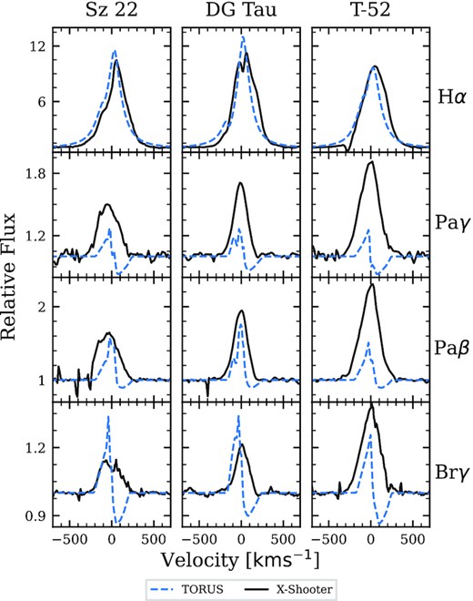
Three of the best cases of the grid matching the observed line profiles. The models have been chosen because they best reproduce the observed H α shape and width. The observed spectra have been adjusted to compensate for each system’s radial velocity.

Parameters of the models presented in Fig. 7.
| Object | Sz 22 | DG Tau | T-52 |
|---|---|---|---|
| |$\log {\dot{M}_{\rm acc}}$| | −8 | −8 | −8 |
| Tacc | 9500 K | 9500 K | 9500 K |
| |$\log {\dot{M}_{\rm sw}}$| | −9 | −9 | −9 |
| Tsw | 10 000 K | 10 000 K | 8000 K |
| Inclination | 80° | 60° | 60° |
| Object | Sz 22 | DG Tau | T-52 |
|---|---|---|---|
| |$\log {\dot{M}_{\rm acc}}$| | −8 | −8 | −8 |
| Tacc | 9500 K | 9500 K | 9500 K |
| |$\log {\dot{M}_{\rm sw}}$| | −9 | −9 | −9 |
| Tsw | 10 000 K | 10 000 K | 8000 K |
| Inclination | 80° | 60° | 60° |
Parameters of the models presented in Fig. 7.
| Object | Sz 22 | DG Tau | T-52 |
|---|---|---|---|
| |$\log {\dot{M}_{\rm acc}}$| | −8 | −8 | −8 |
| Tacc | 9500 K | 9500 K | 9500 K |
| |$\log {\dot{M}_{\rm sw}}$| | −9 | −9 | −9 |
| Tsw | 10 000 K | 10 000 K | 8000 K |
| Inclination | 80° | 60° | 60° |
| Object | Sz 22 | DG Tau | T-52 |
|---|---|---|---|
| |$\log {\dot{M}_{\rm acc}}$| | −8 | −8 | −8 |
| Tacc | 9500 K | 9500 K | 9500 K |
| |$\log {\dot{M}_{\rm sw}}$| | −9 | −9 | −9 |
| Tsw | 10 000 K | 10 000 K | 8000 K |
| Inclination | 80° | 60° | 60° |
A caveat to the direct comparison is that the veiling of the observed lines has not been considered. Whereas the effect of reddening is negated by the continuum normalization, the influence of veiling is not. Nevertheless, Fig. 7 highlights a trend seen in the grid of synthetic spectra. Namely, while our method selects models with similar strengths and widths in H α to that observed, the models fail to reproduce the observed infrared lines. The synthetic infrared lines are too structured and narrow. This trend is presented in more detail in Sections 4.2 and 4.3, and discussed in Section 5.
In the following sections, we present an analysis of the structure (Section 4.1) and the width (Section 4.2) of the ensemble of synthetic line profiles. To best compare the synthetic and observed spectra, we use only a subset of our grid. The models are selected to correspond to the observed H α range. Only models that have an H α HW10 per cent in the range of 60–400 km s−1 are included.
4.1 Reipurth classification
Following the framework given by Reipurth et al. (1996) and outlined in Section 2, the synthetic line profiles were classified using a python routine. The code finds peaks and troughs using a gradient search and uses them to classify the lines with the following order of precedence: IV, I, II, and III. The program defines type IV as being a sub-continuum absorption with no further emission greater than 1 per cent of the peak. If the line contains both red and blue-shifted absorption, the code uses the strongest feature to classify the line. Many profiles have type II, and III features along with type IV. To avoid any classification bias, the spectra from X-shooter are classified using the same order of precedence.
The mean signal-to-noise ratio (SNR) of the X-Shooter spectra are ≈70 for the VIS arm and ≈108 for the NIR. The mean ratio of peak emission to sub-continuum absorption depth for type IV profiles is ≈3 and ≈4 for the optical and infrared lines, respectively. Hence, the sub-continuum absorption features in the synthetic grid are 18–25 times greater than the observed noise level. Consequently, the introduction of noise would not be expected to significantly influence the Reipurth classifications of the synthetic profiles.
Fig. 2 displays the results as hashed bars overlaying the distribution of Reipurth types for the X-Shooter spectra. The H α classifications for the models have the most similar distribution to the observations. IPC profiles are seen in the spectra of one of the 29 T Tauri stars [Reipurth et al. (1996) observed two out of a sample of 43], approximately 3.4 per cent. Whereas 35 per cent of the synthetic H α lines exhibit this morphology. The H α IPC profiles are only present in models that would be classified as Weak Line T Tauri stars, based on the H α 10 per cent width criterion of White & Basri (2003). Blue-shifted sub-continuum absorption is relatively rare for H α and only seen in 7 per cent of the synthetic profiles.
In contrast to the relative agreement seen for H α, the synthetic infrared lines predict a significantly higher frequency of P-Cygni profiles; ≈98 per cent are type IVR or IVB. However, across all three infrared lines, the mean frequency of IPC profiles in the X-Shooter sample is ≈23 per cent and none of the infrared observations exhibit blue-shifted sub-continuum absorption. Comparatively, Folha & Emerson (2001) saw a frequency of type IVR profiles of 34 and 20 per cent for Pa β and Pa γ, respectively. Furthermore, they observed no type IVB profiles in their sample of 50 T Tauri stars.
For the chosen parameters of our model grid, the synthetic line profiles show a much higher occurrence of deep absorption features than is present in our observed sample. We explore possible modifications to the model in Section 4.3 and discuss them further in Section 5.
4.2 Comparison of widths
To analyse the synthetic and observed emission as an ensemble, we calculated the FWHM and the HW10 per cent. A linear interpolation was fitted to the synthetic line profiles so that the FWHM and the HW10 per cent could be measured. We determined the FWHM and the HW10 per cent of the X-Shooter spectra by fitting the line profile with Gaussians rather than a spline to avoid problems with noise and to conform to standard data reduction methods. Two Gaussians were fitted to the emission, and another two Gaussians were used solely to fit the sub-continuum absorption, fitted using a python routine that prioritized reproducing the observed widths.
Fig. 8 shows a plot of the FWHM against the HW10 per cent for the synthetic and observed spectra. Each point corresponds to a different model in our grid, and the colour and size indicate the accretion rate. The cutoff between weak Line and CTTS is shown by the dotted vertical line. For H α, FWHM and the HW10 per cent are strongly correlated for both the observations and models. Both the models and the observed data show that the widths are correlated with the accretion rate. However, the accretion funnel temperature and viewing inclination have significant influence on the width of the model line profiles by scattering in the synthetic line profiles at a given accretion rate. The relationship between the FWHM and HW10 per cent for a Gaussian is ≈1.10, displayed in Fig. 8 by the inclined solid black lines. The observed sample is scattered around this relationship. The synthetic H α spectra have been selected to have a similar range of HW10 per cent as the observations. However, they tend to have a smaller FWHM for a given HW10 per cent. The deviation from the Gaussian FWHM to HW10 per cent relationship is due to Stark broadening. The H α lines have a Voigt profile when Stark broadening is dominant (see Section 3.2.2). The Voigt form has wider wings and a narrower peak than a Gaussian curve. This effect is not observed in the higher lines where Stark broadening is negligible.
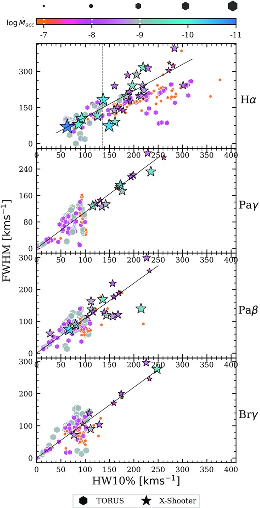
The FWHM versus HW10 per cent for observed (black outlined stars) and torus data (coloured hexagons). The colour and size denote the accretion rate. The vertical dashed line shows the criterion for the H α split between weak line T Tauri stars and CTTS (White & Basri 2003). The diagonal black line is the analytical Gaussian relationship between the FWHM and the HW10 per cent.

For Pa γ and Br γ, the observations exhibit a tight correlation between the FWHM and HW10 per cent. The Pa β observations exhibit a larger scatter, suggesting a divergence away from the Gaussian form and more structure in the line profiles. This is corroborated by the fact that Pa β has the highest frequency (63 per cent) of non-type I profiles (see Fig. 2). In contrast to H α, the FWHM and the HW10 per cent of the higher lines in the observations and models exhibit little correlation with the accretion rate. The models shown in Fig. 8 have been selected so that the range of HW10 per cent widths for H α roughly correspond to the range of the observational data set. However, these models predict widths for the three higher lines that are, on average, much narrower than the observed widths. In general for an accretion rate of |$\log {\dot{M}_{\rm acc}}=-7$| the synthetic lines have a lower ratio of FWHM to HW10 per cent than other accretion rates.
Fig. 9 compares the distributions of synthetic and observed HW10 per cent for all four lines. The distribution of synthetic H α widths is much broader than that observed, simply a result of our parameter grid sampling a relatively uniform coverage of line profiles in this range. However, by constraining our models to a subset of the full grid (see Section 4) the observed and synthetic H α HW10 per cent’s lie in a similar range, with a difference in the respective medians of |$25{~\rm km\,s}^{-1}$|. Conversely for all three of the other spectral lines, the median width of the synthetic line distribution is much narrower than that in the observed sample. The differences in the median value of HW10 per cent for the synthetic and observed infrared line profiles are, Pa|$\beta = 66{~\rm km\,s}^{-1}$|, Pa|$\gamma = 105 {~\rm km\,s}^{-1}$|, and Br|$\gamma = 82 {~\rm km\,s}^{-1}$|. In other words, for a range of models that predict H α line widths in the same range as the observations, the predicted widths in the other lines are systematically too narrow by |${\approx}84{~\rm km\,s}^{-1}$|. In Section 4.3, we explore what modifications can be made to the models to bring these synthetic lines into better agreement with the observed sample.
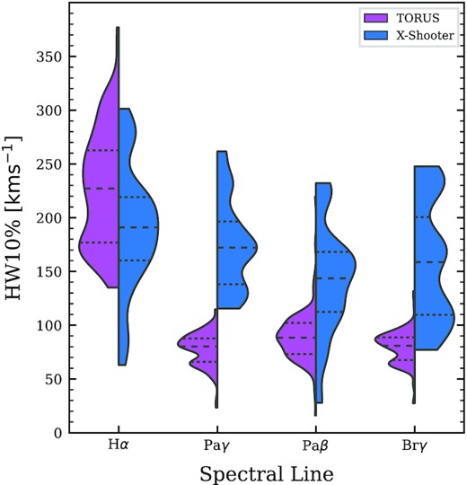
The HW10 per cent distribution of the grid and observations shown for each spectral line. The model data are filtered so that only models with widths such that |$60\le {\rm ~ HW10{{\ \rm per\ cent}}}_{{\rm ~ H}\alpha }\lt 400$| are included. The horizontal dashed lines indicate the 25th percentile, the median, and the 75th percentile of the distributions.

4.3 Modified models
The grid of models does not adequately reproduce the observed frequency of line profile structures (Section 4.1) or the observed range of profile widths (Section 4.2) for the infrared lines. In the following section, we examine the effects of three different model modifications in an attempt to explore what might bring the synthetic and observed line profiles into better agreement. In Section 4.3.1, we examine the effect of introducing turbulent broadening. The influence of rotation on the synthetic lines is introduced in Section 4.3.2. In Section 4.3.3, the widths are re-evaluated, considering only the blue-shifted side, to determine the consequence of the high proportion of sub-continuum absorption on the widths of the line profiles.
4.3.1 Turbulent line broadening
We expect there to be unresolved small-scale motion in the T Tauri system on top of the bulk gas flow, for example, from unsteady accretion and wind flows or from instabilities in the accretion and post-accretion shock gas. However, rather than model the physical processes involved, we assume that the unresolved motions are everywhere in the grid and act like a turbulence, which has a Maxwell–Boltzmann distribution. The effect of Stark broadening on the higher lines is negligible, so an additional broadening from turbulence could increase the synthetic line widths to be more in line with the observations and reduce the frequency of sub-continuum absorption features. To explore the effect of turbulent broadening on the infrared line widths, we introduced a large turbulent velocity component to equation (25). We used a value of vturb = 100 km s−1, which is approximately the largest difference of the median HW10 per cent between the observed and synthetic infrared lines, see Section 4.2. There is little physical justification for a turbulent motion of 100 km s−1, other than it is the required velocity to broaden the ensemble of line profiles sufficiently.
Fig. 10 shows the FWHM versus the HW10 per cent for the Stark and turbulently broadened lines and the Stark-only broadened models. Similar to Fig. 8, the profiles are filtered such that only models with an H α HW10 per cent between 60 and 400 km s−1 are included. The turbulent broadening increases the H α line too much, pushing the median value of the HW10 per cent to ≈320 km s−1. The effect on the higher lines is to bring the range of predicted values to overlap with the observed spectra. The turbulent broadening increases the number of synthetic lines that have HW10 per cent greater than 400 km s−1 by 4 per cent.
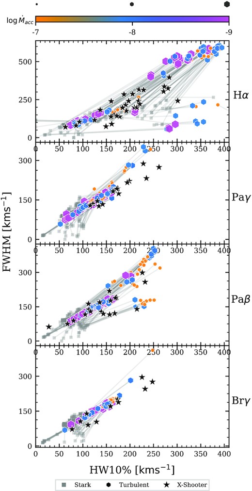
The effect of combining 100 km s−1 of turbulent velocity with the Stark broadening. Grey squares are the original Stark only broadened widths and the coloured hexagons are the Stark and turbulently broadened widths. The grey lines connect the two different models. The accretion rate of the models is indicated by the colour and size of the hexagons. The black stars indicate the widths of the observed T Tauri stars. The added turbulent velocity increases the width of the synthetic profiles bringing the ensemble into better agreement with the observations.

A subset of the turbulently broadened line profiles can be seen in Fig. 11. Similarly to Fig. 6, the spectra are shown for |$\dot{M}_{\rm sw}=0.01~\dot{M}_{\rm acc}$| and Tsw = 8000 K. The figure shows the line profiles organized by accretion rate (columns) and magnetospheric temperature (rows). The effect of the turbulence is to create a boxier profile; steep sides with flat tops. The added turbulent velocity increases the resonant range of the transition wavelength, broadening both the emission and the absorption features. This ‘top-hat’ morphology is not seen in the observed data set. The distribution of the Reipurth classifications is not significantly changed by the turbulence and a high proportion of IPC profiles are still predicted. The boxier profiles increase the ratio between the FWHM and the HW10 per cent, creating a steeper relationship than seen for a Gaussian or a Voigt profile.
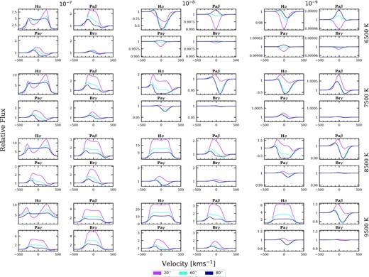
Turbulently broadened torus line profiles arranged by |$\dot{M}_{\rm acc}$| (columns) and Tacc (rows). The y-axis range of Pa γ, Pa β, and Br γ for each subset are shared. The profiles are boxy with a ‘top-hat’ like appearance and the sub-continuum absorption features are broadened.

In conclusion, despite the fact that the turbulent broadening produces an infrared range of line widths in better agreement with the observations, this modification causes the width of the H α lines to be increased too much and the line profiles to become boxy, a morphology not reflected in the observations. There is also little motivation for the turbulent motion to be as high as 100 km s−1. Furthermore, the frequency of sub-continuum absorption is not significantly changed, suggesting that incorporating unresolved small-scale motion into the simulations cannot solely account for the lack of width in the infrared lines.
4.3.2 Rotational line broadening
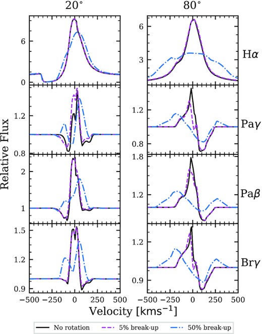
The effect of rotation on line profiles. The profiles are shown for three different rotation rates: no rotation (solid line), 0.05 vbr (pink dashed line), and 0.5 vbr (blue dash–dotted line). The profiles are arranged by viewing inclination (columns) and wavelength (rows). At high rotation rates, the profiles are flattened and broadened. The effect is amplified when viewed from a greater inclination.

The profiles are smoothed and broadened by rotation. However, this effect is negligible unless the rotation is at a significant proportion of the stellar break-up velocity. For example, a rotation velocity of 0.05 vbr had a no effect on H α, whereas for Pa γ and Pa β, the peak intensity was reduced by ≈10 per cent for an inclination of 80°. On the other hand, a rotation rate of 0.5 vbr significantly broadens the synthetic profiles when viewed from a high colatitude. The peaks are shifted away from the rest velocity as the hot, high-density gas in the magnetosphere dominates the emission. Estimates for the observed X-Shooter target’s v sin i and their rotation as a fraction of their break-up velocity are shown in Table 4. V354-Mon has the highest rotation rate in the data set with a velocity of v sin i = 40.9 km s−1, only 11 per cent of the star’s break-up velocity. The rotation rates in our observed data set are not large enough to cause significant line broadening. Therefore, rotational broadening cannot explain the mismatch between the observed and synthetic line widths.
Table showing the rotation rates for the observed X-Shooter stars. References are: (1) Nguyen et al. (2012), (2) Baxter et al. (2009), (3) Frasca et al. (2015), (4) Kounkel et al. (2019), (5) Malo et al. (2014), (6) Manara et al. (2016), (7) Schneider et al. (2018), (8) Manara et al. (2014), (9) McGinnis et al. (2015), and (10) Rugel et al. (2018).
| Name | L* | R* | V sin i | |$\frac{V\sin {i}}{V_{br}}$| | Reference |
|---|---|---|---|---|---|
| [L⊙] | [R⊙] | [km s−1] | |||
| ESO-Ha-562 | 0.12 | 0.8 | 40 | 0.1 | 1,6 |
| IQ-Tau | 0.75 | 1.9 | 14.4 | 0.05 | 1,6 |
| V354-Mon | 1.67 | 1.8 | 40.9 | 0.11 | 2,7 |
| T-33 | 0.69 | 1.1 | 16.5 | 0.04 | 3,6 |
| T-11 | 1.45 | 1.7 | 14.1 | 0.04 | 3,8 |
| VW-Cha | 1.64 | 2.6 | 13 | 0.04 | 1,6 |
| T-6 | 1.17 | 1.5 | 34 | 0.09 | 1,8 |
| CR-Cha | 3.26 | 2.3 | 35 | 0.09 | 1,6 |
| T-52 | 2.55 | 2.0 | 28 | 0.08 | 1,6 |
| T-38 | 0.13 | 0.8 | 18.7 | 0.05 | 1,6 |
| KV-Mon | ∼ | ∼ | 24.25 | ∼ | 4,9 |
| Sz-22 | 0.51 | 1.3 | ∼ | ∼ | 6 |
| T-4 | 0.43 | 1.3 | 12.4 | 0.03 | 1,6 |
| DG-Tau | 1.55 | 2.2 | 24.7 | 0.07 | 1,6 |
| T-23 | 0.32 | 1.8 | 9.6 | 0.05 | 3,6 |
| RECX-12 | 0.23 | 1.4 | 6.4 | 0.03 | 5,10 |
| Cha-Ha-6 | 0.07 | 1.0 | ∼ | ∼ | 6 |
| T-12 | 0.15 | 1.3 | 10.7 | 0.06 | 1,6 |
| CT-Cha-A | 1.5 | 2.2 | 7.8 | 0.02 | 1,6 |
| ESO-HA-442 | ∼ | ∼ | ∼ | ∼ | |
| CHX18N | 1.03 | 1.4 | 26.5 | 0.07 | 1,6 |
| TW-Cha | 0.38 | 1.2 | 11.3 | 0.03 | 1,6 |
| RECX-6 | 0.1 | 0.9 | ∼ | ∼ | 10 |
| T-49 | 0.29 | 1.6 | 8.2 | 0.04 | 1,6 |
| T-35 | 0.33 | 1.2 | 21 | 0.05 | 1,8 |
| T-45a | 0.34 | 1.2 | 12.4 | 0.03 | 1,6 |
| RECX-9 | 0.095 | 1.1 | ∼ | ∼ | 10 |
| T-24 | 0.4 | 1.4 | 10.5 | 0.03 | 1,6 |
| Hn-5 | 0.05 | 0.8 | 7.8 | 0.04 | 1,6 |
| Name | L* | R* | V sin i | |$\frac{V\sin {i}}{V_{br}}$| | Reference |
|---|---|---|---|---|---|
| [L⊙] | [R⊙] | [km s−1] | |||
| ESO-Ha-562 | 0.12 | 0.8 | 40 | 0.1 | 1,6 |
| IQ-Tau | 0.75 | 1.9 | 14.4 | 0.05 | 1,6 |
| V354-Mon | 1.67 | 1.8 | 40.9 | 0.11 | 2,7 |
| T-33 | 0.69 | 1.1 | 16.5 | 0.04 | 3,6 |
| T-11 | 1.45 | 1.7 | 14.1 | 0.04 | 3,8 |
| VW-Cha | 1.64 | 2.6 | 13 | 0.04 | 1,6 |
| T-6 | 1.17 | 1.5 | 34 | 0.09 | 1,8 |
| CR-Cha | 3.26 | 2.3 | 35 | 0.09 | 1,6 |
| T-52 | 2.55 | 2.0 | 28 | 0.08 | 1,6 |
| T-38 | 0.13 | 0.8 | 18.7 | 0.05 | 1,6 |
| KV-Mon | ∼ | ∼ | 24.25 | ∼ | 4,9 |
| Sz-22 | 0.51 | 1.3 | ∼ | ∼ | 6 |
| T-4 | 0.43 | 1.3 | 12.4 | 0.03 | 1,6 |
| DG-Tau | 1.55 | 2.2 | 24.7 | 0.07 | 1,6 |
| T-23 | 0.32 | 1.8 | 9.6 | 0.05 | 3,6 |
| RECX-12 | 0.23 | 1.4 | 6.4 | 0.03 | 5,10 |
| Cha-Ha-6 | 0.07 | 1.0 | ∼ | ∼ | 6 |
| T-12 | 0.15 | 1.3 | 10.7 | 0.06 | 1,6 |
| CT-Cha-A | 1.5 | 2.2 | 7.8 | 0.02 | 1,6 |
| ESO-HA-442 | ∼ | ∼ | ∼ | ∼ | |
| CHX18N | 1.03 | 1.4 | 26.5 | 0.07 | 1,6 |
| TW-Cha | 0.38 | 1.2 | 11.3 | 0.03 | 1,6 |
| RECX-6 | 0.1 | 0.9 | ∼ | ∼ | 10 |
| T-49 | 0.29 | 1.6 | 8.2 | 0.04 | 1,6 |
| T-35 | 0.33 | 1.2 | 21 | 0.05 | 1,8 |
| T-45a | 0.34 | 1.2 | 12.4 | 0.03 | 1,6 |
| RECX-9 | 0.095 | 1.1 | ∼ | ∼ | 10 |
| T-24 | 0.4 | 1.4 | 10.5 | 0.03 | 1,6 |
| Hn-5 | 0.05 | 0.8 | 7.8 | 0.04 | 1,6 |
Table showing the rotation rates for the observed X-Shooter stars. References are: (1) Nguyen et al. (2012), (2) Baxter et al. (2009), (3) Frasca et al. (2015), (4) Kounkel et al. (2019), (5) Malo et al. (2014), (6) Manara et al. (2016), (7) Schneider et al. (2018), (8) Manara et al. (2014), (9) McGinnis et al. (2015), and (10) Rugel et al. (2018).
| Name | L* | R* | V sin i | |$\frac{V\sin {i}}{V_{br}}$| | Reference |
|---|---|---|---|---|---|
| [L⊙] | [R⊙] | [km s−1] | |||
| ESO-Ha-562 | 0.12 | 0.8 | 40 | 0.1 | 1,6 |
| IQ-Tau | 0.75 | 1.9 | 14.4 | 0.05 | 1,6 |
| V354-Mon | 1.67 | 1.8 | 40.9 | 0.11 | 2,7 |
| T-33 | 0.69 | 1.1 | 16.5 | 0.04 | 3,6 |
| T-11 | 1.45 | 1.7 | 14.1 | 0.04 | 3,8 |
| VW-Cha | 1.64 | 2.6 | 13 | 0.04 | 1,6 |
| T-6 | 1.17 | 1.5 | 34 | 0.09 | 1,8 |
| CR-Cha | 3.26 | 2.3 | 35 | 0.09 | 1,6 |
| T-52 | 2.55 | 2.0 | 28 | 0.08 | 1,6 |
| T-38 | 0.13 | 0.8 | 18.7 | 0.05 | 1,6 |
| KV-Mon | ∼ | ∼ | 24.25 | ∼ | 4,9 |
| Sz-22 | 0.51 | 1.3 | ∼ | ∼ | 6 |
| T-4 | 0.43 | 1.3 | 12.4 | 0.03 | 1,6 |
| DG-Tau | 1.55 | 2.2 | 24.7 | 0.07 | 1,6 |
| T-23 | 0.32 | 1.8 | 9.6 | 0.05 | 3,6 |
| RECX-12 | 0.23 | 1.4 | 6.4 | 0.03 | 5,10 |
| Cha-Ha-6 | 0.07 | 1.0 | ∼ | ∼ | 6 |
| T-12 | 0.15 | 1.3 | 10.7 | 0.06 | 1,6 |
| CT-Cha-A | 1.5 | 2.2 | 7.8 | 0.02 | 1,6 |
| ESO-HA-442 | ∼ | ∼ | ∼ | ∼ | |
| CHX18N | 1.03 | 1.4 | 26.5 | 0.07 | 1,6 |
| TW-Cha | 0.38 | 1.2 | 11.3 | 0.03 | 1,6 |
| RECX-6 | 0.1 | 0.9 | ∼ | ∼ | 10 |
| T-49 | 0.29 | 1.6 | 8.2 | 0.04 | 1,6 |
| T-35 | 0.33 | 1.2 | 21 | 0.05 | 1,8 |
| T-45a | 0.34 | 1.2 | 12.4 | 0.03 | 1,6 |
| RECX-9 | 0.095 | 1.1 | ∼ | ∼ | 10 |
| T-24 | 0.4 | 1.4 | 10.5 | 0.03 | 1,6 |
| Hn-5 | 0.05 | 0.8 | 7.8 | 0.04 | 1,6 |
| Name | L* | R* | V sin i | |$\frac{V\sin {i}}{V_{br}}$| | Reference |
|---|---|---|---|---|---|
| [L⊙] | [R⊙] | [km s−1] | |||
| ESO-Ha-562 | 0.12 | 0.8 | 40 | 0.1 | 1,6 |
| IQ-Tau | 0.75 | 1.9 | 14.4 | 0.05 | 1,6 |
| V354-Mon | 1.67 | 1.8 | 40.9 | 0.11 | 2,7 |
| T-33 | 0.69 | 1.1 | 16.5 | 0.04 | 3,6 |
| T-11 | 1.45 | 1.7 | 14.1 | 0.04 | 3,8 |
| VW-Cha | 1.64 | 2.6 | 13 | 0.04 | 1,6 |
| T-6 | 1.17 | 1.5 | 34 | 0.09 | 1,8 |
| CR-Cha | 3.26 | 2.3 | 35 | 0.09 | 1,6 |
| T-52 | 2.55 | 2.0 | 28 | 0.08 | 1,6 |
| T-38 | 0.13 | 0.8 | 18.7 | 0.05 | 1,6 |
| KV-Mon | ∼ | ∼ | 24.25 | ∼ | 4,9 |
| Sz-22 | 0.51 | 1.3 | ∼ | ∼ | 6 |
| T-4 | 0.43 | 1.3 | 12.4 | 0.03 | 1,6 |
| DG-Tau | 1.55 | 2.2 | 24.7 | 0.07 | 1,6 |
| T-23 | 0.32 | 1.8 | 9.6 | 0.05 | 3,6 |
| RECX-12 | 0.23 | 1.4 | 6.4 | 0.03 | 5,10 |
| Cha-Ha-6 | 0.07 | 1.0 | ∼ | ∼ | 6 |
| T-12 | 0.15 | 1.3 | 10.7 | 0.06 | 1,6 |
| CT-Cha-A | 1.5 | 2.2 | 7.8 | 0.02 | 1,6 |
| ESO-HA-442 | ∼ | ∼ | ∼ | ∼ | |
| CHX18N | 1.03 | 1.4 | 26.5 | 0.07 | 1,6 |
| TW-Cha | 0.38 | 1.2 | 11.3 | 0.03 | 1,6 |
| RECX-6 | 0.1 | 0.9 | ∼ | ∼ | 10 |
| T-49 | 0.29 | 1.6 | 8.2 | 0.04 | 1,6 |
| T-35 | 0.33 | 1.2 | 21 | 0.05 | 1,8 |
| T-45a | 0.34 | 1.2 | 12.4 | 0.03 | 1,6 |
| RECX-9 | 0.095 | 1.1 | ∼ | ∼ | 10 |
| T-24 | 0.4 | 1.4 | 10.5 | 0.03 | 1,6 |
| Hn-5 | 0.05 | 0.8 | 7.8 | 0.04 | 1,6 |
4.3.3 Blue-shifted emission
Over 80 per cent of the infrared emission lines from the models have IPC features, much more frequent than the ∼23 per cent of observed line profiles with IPC profiles (Section 2). The red-shifted sub-continuum absorption makes the line profiles narrower. Thus, if our model were modified to reduce the frequency of IPC profiles, we expect that the average line widths will also increase. A possible mechanism for removing the red-shifted absorption is introducing a non-axisymmetric accretion flow where the accreting column only periodically intersects with the line of sight. For example, Esau, Harries & Bouvier (2014) used a non-axisymmetric accretion flow to reproduce the Balmer variations seen for AA Tau successfully; this effect is discussed further in Section 5.
To estimate how much the IPC absorption might be affecting the line widths in our models, we calculated the HW10 per cent values using only the blue side of each synthetic line profile (HW10 per centBlue). We employed a linear interpolation of the line that was blue shifted from the peak to determine values of the profile width. Fig. 13 shows the HW10 per centBlue versus the true HW10 per cent. The diagonal line (black dashed) shows the one to one ratio; points below the diagonal indicate the width decreased when considering only the blue side. The points are coloured, indicating the model’s inclination. For a viewing angle of 20°, the majority of line widths decreased when solely considering the blue-shifted emission. The blue sides of these modelled lines are narrower than the red due to the strong blue-shifted absorption from the stellar wind, which lies along the line of sight at this inclination. Type IV profiles are rare in our observed data set, and so to focus on the broadening effect they are excluded from the following analysis. Fig. 13 shows the distribution of width-change (Δ HW10 per cent) as a series of histograms. The mean shift for all the models with an inclination of either 60° or 80° is |$49{~\rm km\,s}^{-1}$|. When only models with a very low mass-loss rate (|$0.001\dot{M}_{\rm acc}$|) are considered the average increase in width is |${\approx}50{~\rm km\,s}^{-1}$| for inclinations of 60° and 80°.
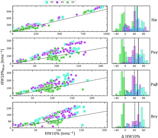
Comparison of the true HW10 per cent and the half-width measured for only blue-shifted emission (HW10 per centBlue). The dashed diagonal line has a gradient of unity; points above it are broader when only the blue-shifted emission is considered. The colour and style of the points denote the model inclination. Plotted on the right are histograms showing the difference of the two measured widths. The vertical lines indicate the respective means: 20° dotted, 60° dashed, and 80° solid.

The above analysis suggests that if the models were modified in some way to reduce the prevalence of IPC absorption, the synthetic line profiles would become significantly wider by an average of |${\approx}49{~\rm km\,s}^{-1}$|. An average increase of |${\approx}84{~\rm km\,s}^{-1}$| (Section 4.2) is needed to shift the HW10 per cent of the synthetic infrared lines into agreement with the observations. Therefore, while this effect cannot account for the whole disparity of widths on its own, when combined with other mechanisms, such as turbulence and rotation, it may be sufficient.
5 DISCUSSION
A significant caveat to our comparison of the observed and synthetic line profiles is the possibility that our observed data set is incongruous and not representative of the consensus of T Tauri stars. However, our sample of 29 stars appears to be consistent with other observational data sets. For instance, the sample has a similar fraction of Reipurth classes to the distributions reported by Reipurth et al. (1996) for H α and Folha & Emerson (2001) for Pa β and Br γ. Additionally, the Pa β and Br γ line peaks are slightly blue-shifted in agreement with Folha & Emerson (2001), even though the mean FWHM of our line profiles is smaller than the mean FWHM reported by Folha & Emerson (2001).
A second caveat is that our grid of synthetic line profiles was not adjusted to attain an agreement with any particular observation and a singular stellar mass, radius, and temperature were used. Broadly speaking, the synthetic line profile morphology is determined by the geometry, accretion rate, and temperature of the magnetosphere. Accordingly, our grid was designed to encompass the broad range of parameters predicted for T Tauri accretion and outflow (e.g. Hartmann et al. 1994; Muzerolle et al. 1998, 2001; Kurosawa et al. 2006; Lima et al. 2010; Kurosawa & Romanova 2012). In turn, our T Tauri sample has an extensive range of accretion rates and stellar parameters, making it an appropriate initial data set for a comparison with the ensemble of synthetic spectra.
Our models predict a greater number of H α IPC profiles than observed. However, our grid of models can reproduce the observed fraction of H α Reipurth types, after the lines classified as Weak Line T Tauri stars (≈40 per cent) are removed. By removing the Weak Line T Tauri models, we discard the H α models that contain red-shifted sub-continuum absorption. Hence, for our model grid, IPC profiles are only produced by models that would be classified as Weak Line T Tauri stars. This result is substantiated by Kurosawa et al. (2006) who demonstrated that H α IPC profiles were only produced in ≈5 per cent of their sample. Moreover, in these cases, the accretion rate was low enough that the lines would be consistent with a weak line T Tauri classification.
The same models that correctly reproduce the observed H α Reipurth types predict a very high frequency of IPC profiles for Pa β, Pa γ, and Br γ. For H α, Stark broadening smooths out the synthetic spectra, masking absorption features (Muzerolle et al. 2001). However, for the higher lines, the effect of Stark broadening is negligible at the temperatures and densities expected in T Tauri accretion. A possible reason for the dearth of observed IPC profiles is non-axisymmetric accretion flow. A magnetic obliquity from the stellar pole could cause the accretion funnel to form ‘curtains’ that rotate with the star. IPC profiles would then be seen intermittently when the accretion curtain intersects with the line of sight. Observations support this effect; for example, McGinnis et al. (2020) measured a magnetic obliquity of |$18^{\circ }{}^{+8}_{-7}$| for DK Tau and observed an IPC profile for two of the eight epochs. Accretion funnel ‘curtains’ have also been explored in radiative transfer studies. For instance, Symington et al. (2005) used a 3D non-axisymmetric model, to reproduce some of the observed variability seen in T Tauri stars, but in general, the models produced results that were too variable. Esau et al. (2014) successfully modelled variable Balmer emission from AA Tau with a non-axisymmetric accretion model and Alencar et al. (2012) reproduced Balmer lines from V2129 Oph over several stellar rotational cycles. Further analysis of T Tauri time-series spectroscopic surveys would be helpful in better quantifying the variability of IPC profiles across multiple wavelengths.
In addition to the red-shifted features from the magnetosphere, some interesting blue-shifted detail are created by the stellar wind. The stellar wind produces the characteristic broad sub-continuum absorption as noted by Kurosawa et al. (2011). P-Cygni features occur in ≈13 per cent of the synthetic profiles, and ≈10 per cent of those do not contain red-shifted sub-continuum absorption. On the other hand, P-Cygni profiles are very rare in our observations, with none exhibited for the infrared lines. The infrared lines are optically thinner than H α, and therefore, less sensitive to the lower density wind. P-Cygni profiles were also noted to be rare by Folha & Emerson (2001) and Edwards et al. (2006). Why these mass outflow signatures are scarce in observations could be a matter of geometry, temperature, or mass-loss rate. Geometry should significantly reduce the frequency of fast wind absorption, since those winds are likely to be collimated (Edwards et al. 2006). Lima et al. (2010) showed that for H α a mass-loss rate from the inner disc of at least 10−9 M⊙ yr−1 was needed for blue-shifted absorption features to show. However, for a polar stellar wind, our models produced H α blue-shifted sub-continuum absorption for mass-loss rates as low as 10−12 M⊙ yr−1. Additionally, our results suggest that the frequency of synthetic P-Cygni profiles depends on the ratio of the mass-loss to mass accretion rate, not the mass-loss rate alone, because higher accretion rates increase the magnetospheric and hotspot emission that masks the absorption from the wind.
Another factor seen in Section 4.2 is that the infrared line widths (FWHM and HW10 per cent) of the synthetic and observed data sets do not agree. Models that produce H α profiles that lie within the observed range create Paschen and Brackett spectra that are too narrow by ≈84 km s−1. Alencar & Basri (2000) suggested that rotation and turbulence may play an important role in the formation of the infrared line profiles. In agreement with Muzerolle et al. (2001), our results demonstrated that stellar rotation has a negligible effect on the line widths at the rotation rates seen in our observed sample. Furthermore, the level of turbulent motion needed to broaden the synthetic lines sufficiently to account for the difference in width of the synthetic infrared and H α lines is high, |${\approx}100{~\rm km\,s}^{-1}$|. Not only is there no obvious physical justification for such a large value of turbulence, but the spectra produced are broad and flat-topped, a morphology not seen in observations.
In addition to turbulence and rotation, we attempted to quantify the reduction in the width of the spectra due to red-shifted absorption, by calculating the width using only the blue-shifted emission; an approach similar to that adopted by Alencar et al. (2012) to compensate for poorly fitting red-shifted absorption. As expected (Bouvier et al. 2007; Alencar et al. 2012), our analysis suggested that a significant change in the model geometry that removed the IPC absorption, such as non-axisymmetric accretion, could account for a substantial increase in the infrared line widths. Alone, such a method may not be sufficient to account for the disparity between synthetic and observed hydrogen profiles. However, if the models were to include some combination of stellar rotation, turbulence, and non-axisymmetric accretion, the synthetic profiles may be shifted into accord with the observations. Conversely, Folha & Emerson (2001) showed that, for their sample of Pa β and Br γ T Tauri spectra, the FWHM of Reipurth type I and type IVR profiles were not significantly different. This would indicate that spectra with inverse P-Cyni profiles are generally broader than those without or that the sub-continuum absorption does not significantly narrow the spectra. However, there is not a sufficient population of type IVR’s in our sample to confirm this result.
Another factor not taken into account is the line emission from the accretion shock region. This work treats the accretion shock zone as a blackbody heated by the release of gravitational potential energy that adds to the continuum. However, the accretion regions will also have line emission (e.g. Dodin 2018) that will contribute to the observed spectra. A complete radiative equilibrium treatment of the shock region and magnetosphere is necessary to constrain this effect fully, which requires the development of a self-consistent theory of the heating and cooling mechanisms in the magnetosphere.
6 CONCLUSIONS
We presented a grid of synthetic T Tauri line profiles, computed using the radiative transfer code torus. Our models used the magnetospheric model originally developed by Hartmann et al. (1994) and further developed by Muzerolle et al. (1998, 2001), Symington et al. (2005), Kurosawa et al. (2006), Lima et al. (2010), and Kurosawa et al. (2011). Our models also included a polar stellar wind launched from the star’s surface, a more realistic development to stellar wind used by Kurosawa et al. (2011). We compared our ensemble of models to the spectra of 29 T Tauri stars. The medium-resolution spectra covered a broad range of wavelengths that allowed us to simultaneously compare H α, Pa β, Pa γ, and Br γ lines. We drew the following conclusions:
The observations exhibited similar Reipurth classifications, widths, and mean line centres to those seen in other studies (e.g. Folha & Emerson 2001; Reipurth et al. 1996; Edwards et al. 2006).
For H α, our grid of synthetic line profiles was able to reproduce the observed distribution of Reipurth classifications and line widths. However, for the same models, the infrared lines could not reproduce the observed emission. The modelled lines were too narrow by |${\approx}84{~\rm km\,s}^{-1}$| and the majority (≈90 per cent) had IPC profiles.
We explored the effect of rotation and turbulence and determined that they could not sufficiently broaden the synthetic infrared line profiles or remove the IPC features. The red-shifted sub-continuum absorption was determined to narrow the HW10 per cent of the lines by ≈49 km s−1.
The polar stellar wind produced the characteristic broad P-Cygni profiles as suggested by Kurosawa et al. (2011). Our models produced blue-shifted sub-continuum absorption with mass-loss rates as low as 10−12 M⊙ yr−1. Furthermore, our results suggested that the frequency of P-Cygni profiles depends on the ratio of the mass-loss to mass accretion rate; the increased emission from higher accretion rates masks the blue-shifted absorption.
Looking forward, future radiative transfer models should include 3D non axi-symmetric models and work to obtain a better match to the observed red-shifted absorption and emission features. The radiative transfer models should be compared to higher resolution observational spectra and include a more complete analysis that takes into account for veiling and extinction effects. Furthermore, the radiative transfer models of T Tauri stars contain a plethora of free parameters. The addition of further constraints on the geometry and temperature of these models is vital if radiative transfer models are to be used as a comprehensive diagnostic tool of T Tauri spectra.
ACKNOWLEDGEMENTS
The authors acknowledge funding from the European Research Council (ERC) under the European Union’s Horizon 2020 research and innovation program (grant agreement no. 682393; AWESoMeStars: Accretion, Winds, and Evolution of Spins and Magnetism of Stars; http://empslocal.ex.ac.uk/AWESoMeStars).
This research has made use of the services of the European Southern Observatory (ESO) Science Archive Facility. Our research is based on observations collected at the European Southern Observatory under ESO programme 084.C-1095(A).
The authors would like to acknowledge the use of the University of Exeter High-Performance Computing facility in carrying out this work.
This research has made use of the SIMBAD data base, operated at Centre de Données astronomiques de Strasbourg, France (Wenger et al. 2000).
We thank the developers of the python packages, pandas (Reback et al. 2020) and matplotlib (Hunter 2007) that were used for data analysis and creating the figures in this work.
We thank the anonymous referee who provided us with comments and suggestions that improved the clarity of the manuscript.
DATA AVAILABILITY
The VLT/X-Shooter observations are available in the ESO Science Archive Facility at https://archive.eso.org/scienceportal/home under the program ID 084.C-1095(A). The radiative transfer data underlying this article were generated using the code torus that can be found at http://www.astro.ex.ac.uk/people/th2/torus_html/homepage.html.