 https://orcid.org/0000-0003-4342-6215
Abstract
Speculations on hybridization among wild cycads are abundant, but empirical evidence of hybridization in cycad evolution is almost non-existent and the evolutionary consequences of hybridization in cycads have not been discussed. Previously, Zamia katzeriana was hypothesized to have a hybrid origin between two sympatric species: Z. splendens and Z. loddigesii. In this study, we aimed to reveal whether such a hypothesis is confirmed. Variation in 12 microsatellite loci, 12 morphological traits and environmental niche of ten populations representing the three species was examined. Gene flow and scenarios of demographic history were tested. Ecological niche models were reconstructed to examine present and past niche availability of the two putative parental species. Correlations between genetic, morphological, environmental and geographical distances were tested. We found that Z. katzeriana diverged from Z. splendens without experiencing admixture with its sympatric congeners. However, gene flow between Z. splendens and Z. loddigesii has occurred in one locality. The niches of the two latter species have overlapped since the Last Glacial Maximum, when admixture probably occurred. However, the admixed populations do not resemble Z. katzeriana. These results confirm that Z. katzeriana did not originate from hybridization between Z. splendens and Z. loddigesii.
INTRODUCTION
Hybridization, defined in evolutionary biology as the crossing between individuals from separate populations with disparate adaptive norms (Stebbins, 1959) or distinct heritable characters (Harrison, 1990), plays important roles in demographic dynamics, species delimitation and the origin of new species (Rieseberg et al., 2003; Feliner et al., 2017). Speciation by means of hybridization may produce either polyploid or homoploid new lineages (Petit, Bretagnolle & Felber, 1999; Gross & Rieseberg, 2005; Wood et al., 2009; Feliner et al., 2017, Fujiwara et al., 2022), and the ecological mechanisms underlying such a process may be explained by scenarios of secondary contact (Stebbins, 1985). If two species enter in temporal sympatry, hybrids may be formed and, if reproductive isolation is achieved, it is expected that hybrids will occupy an intermediate niche between the two parental species to avoid niche competition (Buerkle et al., 2000). Thus, to determine whether a species is a product of hybridization, it is important to consider both ecological and historical factors involved in the distinction of the studied species.
Cycads comprise 370 species of gymnosperms from tropical or subtropical regions worldwide (Calonje, Stevenson & Osborne, 2022). Horticultural hybridization has continuously demonstrated that the crossing between two well-defined cycad species (and even between genera) is possible (Chamberlain, 1926; Norstog, 1987). This suggests that the intrinsic reproductive barriers in cycads are rather weak, and the hypothesis of speciation via hybridization in nature in cycads therefore appears reasonable. However, empirical evidence of hybridization among natural cycad populations is almost non-existent. Early in 1959, Van Der Walt (1959) proposed that natural hybridization between Encephalartos altensteinii Lehm. and E. lehmannii Lehm. occurred, as they are sympatric in Gqeberha (former Port Elizabeth), South Africa. F1 crosses in Encephalartos Lehm. can be produced through artificial means (Vorster, 1986), but the occurrence of hybrids in nature remains untested. Johnson (1963) suggested that Macrozamia communis L.A.S.Johnson, Macrozamia secunda C.Moore and Macrozamia pauli-guilielmi Hill & Muell. ex F.Muell. were likely to hybridize each other in New South Wales, Australia, given their morphological resemblance and geographical closeness. The hypothesis on the existence of hybridization between wild populations of these mentioned species also remains untested.
The hypothesis of speciation via hybridization has been invoked in the Neotropical genus Zamia L. (Zamiaceae) to explain the intermediate morphological variation or subtle differentiation among species. For example, Norstog (1987, 1990) conducted experiments to demonstrate morphological intermediacy in F1 and F2 crosses between Zamia furfuracea L.f. with Zamia spartea A.DC. Likewise, Vovides (1988) reported the existence of individuals with intermediate morphology and epidermal anatomy features between Zamia loddigesii Miq. and Z. furfuracea in coastal southern Veracruz, Mexico, which might suggest that genetic admixture has occurred in this location. Schutzman (2004) suggested that possible cases of hybridization might happen among Zamia neurophyllidia D.W.Stev., Zamia skinneri Warsz., Zamia prasina W.Bull and Zamia variegata Warsz. Pérez-Farrera et al. (2012) mentioned that Zamia grijalvensis Pérez-Farr., Vovides & Mart.-Camilo, given its leaf and leaflet morphology, might have been originated from the hybridization between Z. loddigesii and some lineage derived from Zamia splendens Schutzman. Although the hypothesis of hybridization is plausible in these cases, these studies lack the genetic evidence necessary to test scenarios of admixture among species.
To date, only a few studies have demonstrated that genetic admixture among cycad species in the wild is possible. Tao et al. (2021), using phylogenetic methods, detected patterns of ancient admixture among species of Cycas L. in China, particularly between Cycas dolichophylla K.D.Hill, T.H.Nguyên & L.K.Phan and Cycas szechuanensis W.C.Cheng & L.K.Fu and between Cycas dolichophylla and the ancestor of Cycas taiwaniana (Carruth.) J.Schust. and Cycas changjiangensis N.Liu. In the study by Meerow et al. (2012a), using the private allele method (Slatkin, 1985), the authors estimated low levels of gene flow among Zamia pumila L., Zamia erosa O.F.Cook & G.N.Collins and Zamia portoricensis Urb.; the numbers of migrants per generation (Nm) were barely >1 in a few interspecies comparisons, but the topic of hybridization was not discussed in that study. A possible case of cycad hybridization was tested later by Pérez-Farrera et al. (2016), demonstrating that Zamia katzeriana (Regel) E.Rettig (2n = 16) has overall morphological and anatomical intermediateness between Z. splendens (2n = 16) and Z. loddigesii (2n = 18) (chromosome numbers as reported by Norstog, 1980; Moretti et al., 1991; Nicolalde-Morejón, Vovides & Stevenson, 2009). Zamia splendens has wide oblong leaflets and Z. loddigesii has linear narrow leaflets; Z. katzeriana appears to have an intermediate variation between those two species (Fig. 1), and this was used as an argument to propose the idea of its hybrid origin by Pérez-Farrera et al. (2016). Certainly, cycad crosses usually show intermediate morphological trait variation (Chamberlain, 1926; Norstog, 1987, 1990). However, although morphological intermediateness might be one possible evidence of hybrid origin (Hardig et al., 2000), understanding the genetic structure, demographic history and the ecological factors of the species involved is crucial in understanding whether speciation via hybridization in cycads has actually occurred (Rieseberg, 1997). In addition, the putative parental species differ in the number of chromosomes: Z. splendens is 2n = 16 and Z. loddigesii is 2n = 18. Although we do not preclude the possibility of chromosome number variation among populations, as it seems that Zamia spp. are variable (Norstog, 1980; Moretti et al., 1991; Olson and Gorelick, 2011), it would be difficult to explain a chromosomal rearrangement to produce viable and fertile Z. katzeriana with 2n = 16. This previous knowledge challenges the idea of hybrid speciation in Z. katzeriana. Therefore, the hybrid origin of Z. katzeriana needs to be evaluated, and this study aims at testing whether Z. katzeriana originated from hybridization between Z. splendens and Z. loddigesii.
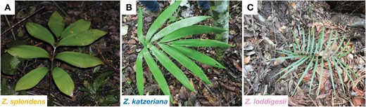
The three species analysed in this study: A, Zamia splendens; B, Z. katzeriana and C, Z. loddigesii. Photographs: the authors.

The most recent phylogenetic study of Zamia (Calonje et al., 2019) resolved the position of Z. splendens in a clade (‘Mesoamerica’ clade, ‘Mexico’ subclade) together with Z. loddigesii. However, they are not sister species since there are several Zamia spp. phylogenetically closer to each. In the subclade ‘Purpurea’, Z. splendens grouped with Zamia lacandona Schutzman (2n = 16, 17, 18), Z. grijalvensis (2n = 19, 20), Zamia purpurea Vovides, J.D.Rees & Vázq.Torres (2n = 16) and Zamia cremnophila Vovides, Schutzman & Dehgan (2n = 16), which are species with broad, scarce leaves, mainly living in primary and secondary rainforests. In the subclade ‘Furfuracea’, Z. loddigesii grouped with other species that have narrow, abundant leaves, occurring at more open, less humid areas [e.g. Z. furfuracea (2n = 18), Z. spartea (2n = 18)]. Zamia katzeriana was not included in the study by Calonje et al. (2019), but based on their morphological similarities, Z. katzeriana is the closest relative of Z. splendens. Actually, such a similarity has confused the taxonomic delimitation between the two species, and the concept of Z. splendens was merged with the concept of Z. katzeriana by Nicolalde-Morejón et al. (2008). However, Pérez-Farrera et al. (2016) separated both species, demonstrating that Z. katzeriana, despite having an overall similarity with Z. splendens, has narrower and fewer leaflets, erect female cones and less shiny leaves. There is also a suite of anatomical traits that significantly differ from Z. splendens (Vovides et al., 2020).
Zamia splendens and Z. katzeriana are both endemic to the rainforests of Chiapas, south-eastern Veracruz and Tabasco, Mexico, at elevations <1000 m a.s.l. Zamia loddigesii has a wider distribution range, occurring in Tamaulipas and Veracruz on the western side of the Isthmus of Tehuantepec, and Tabasco and Chiapas on the eastern side. Zamia loddigesii is sympatric with the other two species at their southernmost distribution ranges, around El Ocote Biosphere Reserve in Ocozocoautla, and San Fernando, Chiapas (Fig. 2A, B). In such areas, their populations do not co-exist, but are separated by up to 2 km. However, it has been documented that pollinators of cycads (beetles of the families Curculionidae or Erotylidae) may disperse pollen by up to several kilometres (Yang and Meerow, 1996), and hybridization is therefore plausible. The weevil species Rhopalotria (Allocorynus) furfuracea has been found to be associated with both Z. loddigesii and Z. splendens (Toon et al., 2020), but there is no information about the possible pollinators for Z. katzeriana. However, the occurrence of male and female strobili in the three species overlaps from May to September (Pérez-Farrera et al., 2016), suggesting similar reproductive phenologies and the possibility that pollinators are shared among species. The distribution ranges of the three cycads and their occurrences in the field suggest that Z. splendens and Z. katzeriana prefer shady humid places, whereas Z. loddigesii can occur in dry, exposed environments, which might explain its wide distribution range in south-eastern to north-eastern Mexico (Fig. 2B).
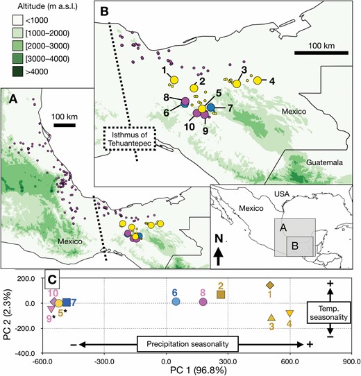
Geographical distribution of three Zamia species analysed. A, The distribution range of Z. loddigesii (pink dots) spans from south-eastern to north-eastern Mexico across the Isthmus of Tehuantepec (dotted line). At the eastern side of the Isthmus, the range of Z. loddigesii overlaps with the distribution of Z. splendens (yellow dots) and Z. katzeriana (blue dots). B, Distribution of the analysed Zamia species from the eastern side of the Isthmus of Tehuantepec. Populations 1–10 were evaluated in genetic and morphological analyses. The population numbers correspond to the localities listed in Table 1. C, Principal component analysis plot that shows the environmental variation among the ten analysed populations. The two main components represent 96.8 and 2.3% of the total variation, each respectively representing precipitation and temperature seasonality. Asterisks indicate populations that showed patterns of admixture in genetic analyses.

Populations of three Zamia species examined in this study
| Populations | Species | Samples for genetic analyses | Samples for morphological analyses | Locality | Herbarium vouchers representing the populations |
|---|---|---|---|---|---|
| Pop1 | Z. splendens | 20 | 19 | Las Choapas, Veracruz | Las Choapas, 195 m, 11 January 2004, R. Martínez-Camilo & R. Martínez-Meléndez 825 (HEM). |
| Pop2 | Z. splendens | 20 | 18 | Huimanguillo, Tabasco | Huimanguillo, 480 m, 8 August 2015, M.A. Pérez-Farrera 3032 (HEM). |
| Pop3 | Z. splendens | 20 | 15 | Tapijulapa, Tabasco | Teapa, 340 m, 16 April 1996, M.A. Pérez-Farrera 899 (HEM) |
| Pop4 | Z. splendens | 10 | 16 | Salto de Agua, Chiapas | Salto de Agua, 960 m, 10 November 2016, M.A. Pérez-Farrera 3472 (HEM) |
| Pop5 | Z. splendens | 15 | 18 | Selva El Ocote, Chiapas | Ocozocuautla, 900 m, 5 November 1971, D.E. Breedlove & A.R. Smith 21832a, 400 m, 32579 (CAS) |
| Pop6 | Z. katzeriana | 18 | 17 | Selva El Ocote, Chiapas | Ocozocoautla, Campamento El Encajonado, Reserva El Ocote, 195 m, 15 July 2016, M.A. Pérez-Farrera 3457 (HEM); 657 m, 20 January 2016, H. Gómez Domínguez 3410 (HEM) |
| Pop7 | Z. katzeriana | 13 | 12 | San Fernando, Chiapas | San Fernando, 710 m, 18 May 1988, D.E. Breedlove; Mona Bourell 68259 (CAS); 850 m, 29 April 1995, M.A. Pérez-Farrera 294 (HEM); 680 m, 29 April 1995, A. Vovides 1266 (XAL); 685 m, F. Nicolalde & M.A. Pérez-Farrera 1420 (XAL); 650 m, M.A. Pérez-Farrera s.n. (XAL). |
| Pop8 | Z. loddigesii | 17 | 15 | Selva El Ocote, Chiapas | Ocozocoautla, Campamento Rabasa, Reserva El Ocote, 1253 m, 3 May 2016, H. Gómez Domínguez 3727 (HEM) |
| Pop9 | Z. loddigesii | 18 | 12 | Ocozocoautla, Chiapas | Ocozocoautla, 800 m, 28 April 1995, M.A. Pérez-Farrera 290 (HEM) |
| Pop10 | Z. loddigesii | 19 | 20 | Cintalapa, Chiapas | Cintalapa, Los Bordos, 920 m, April 2015, H. Gómez Domínguez s.n. (HEM) |
Genetic analyses using hypervariable molecular markers could be effective to untangle the relationships among populations in such a complex geographical and ecological region; additionally, genetic data can be used to reconstruct the demographic history and the ancestral-descent relationships among the population groups involved. The hypothesis that Z. katzeriana is a product of the hybridization would be substantiated if (1) genetic variation of Z. katzeriana is intermediate between Z. splendens and Z. loddigesii; (2) if historical or recent gene flow can be detected between Z. katzeriana and both species, Z. splendens and Z. loddigesii; (3) if any putative hybrid between Z. splendens and Z. loddigesii have the same (or at least highly resembling) morphology of the individuals recognized as Z. katzeriana; and (4) if a possible event of secondary contact can be detected between Z. splendens and Z. loddigesii in the area where Z. katzeriana now occurs. Therefore, in this study, we aimed to test the species delimitation among the three Zamia spp. and evaluate gene flow to determine whether hybridization has occurred among them. The results of this research are expected to clarify the occurrence and the consequences of hybridization in cycad evolution. In addition, the results would add evidence concerning the taxonomic distinction between Z. splendens and Z. katzeriana and provide information on the levels of genetic diversity in the three species; the latter is especially necessary for Z. katzeriana, a species considered Endangered (EN) in the IUCN Red List (Pérez-Farrera & Vovides, 2022).
MATERIAL AND METHODS
DNA analyses: sampling and production of data
We analysed 170 samples belonging to five populations of Z. splendens, two of Z. katzeriana and three populations of Z. loddigesii (Table 1). Total genomic DNA was extracted from fresh leaflets with the CTAB method (Doyle & Doyle, 1987). Twelve nuclear SSR loci originally produced for Zamia integrifolia L.f. (Zam05: Meerow et al., 2012a; Zam16, Zam53, Zam58, Zam60 and Zam62: Meerow et al., 2012b, and Zam28, Zam29, Zam32, Zam35, Zam40 and Zam45: Meerow & Nakamura, 2007) were amplified using the primers given in the cited papers (Supporting Information, Table S1). Polymerase chain reactions were prepared in volumes of 25 µL, consisting of 1.25 U of GoTaqFlexi DNA Polymerase (Promega), 3 mM MgCl2, 10 µM for each primer, 1 × Green GoTaq Flex Buffer PCR and 1 µL of template DNA. PCR conditions consisted of one cycle of 5 min at 94 °C, 35 cycles of 1 min at 94 °C, 30 s at temperature of alignment (temperature of each primer pair is specified in Supporting Information, Table S1) and 1 min at 72 °C, and a final extension of 10 min at 72 °C. Genotyping was performed in a ABI3730XL sequencer by Macrogen, Inc. (South Korea). Each locus was genotyped separately. Fragment sizes were calculated with the software GeneMapper v.4.0 (Applied Biosystems, Inc., Foster City, CA, USA) by comparison to an internal molecular marker standard of 400 base pairs. The locus Zam29 showed no polymorphisms, and it was excluded from subsequent analyses.
Integrity of data
The program MicroChecker v.2.2.3 (Van Oosterhout et al., 2004) was used to identify possible scoring error due to stuttering, allele dropout or null alleles in the loci analysed for all populations except populations 1, 4 and 8 (due to low sampling). The Hardy–Weinberg equilibrium test was also conducted for each locus in each population with GeneAlex v.6.5 (Peakall & Smouse, 2006). The outlier loci detection test implemented in the software BayeScan (Foll & Gaggiotti, 2008) was used to estimate whether the employed loci are under selection. This analysis consisted of 100 000 pilot runs, 50 000 burn-in periods and 100 prior odds.
Estimation of genetic diversity parameters
Genetic diversity parameters (observed, expected and unbiased expected heterozygosity, number of alleles, number of effective alleles and the fixation F-index), the FST genetic differentiation among populations and phi-values calculated with 999 bootstraps were estimated in GenAlex (Peakall & Smouse, 2006). FST is informative about the differentiation among populations and does not make assumptions on the mutation models of the microsatellites (Holsinger & Weir, 2009). On the other hand, phi-values are based on the distances among alleles (Holsinger & Weir, 2009), and the calculation in GenAlex allows resampling, thus being informative about the differentiation significance. A graphical representation of the FST values among populations was constructed using the software MEGAX (Kumar et al., 2018). GenAlex was also used for calculation of the pairwise distance matrices of mean pop codom-genotypic genetic distances among individuals and among populations. These distance matrices were used to construct principal coordinate analyses (PCAs) to calculate the dispersion of individuals/populations among the two main components that summarized the total variation. Analysis of molecular variance (AMOVA) (Excoffier, Smouse & Quattro, 1992) was performed using 999 permutations, considering ten populations hierarchically categorized in three species.
Population genetic clustering
To estimate population genetic clustering, we used the Bayesian method implemented in STRUCTURE v.2.3.4 (Pritchard, Wen & Falush, 2010) with the admixture model, considering correlated allele frequencies (with default settings), and considering the population membership as prior information (Hubisz et al., 2009). We tested clustering K = 1–10, with ten iterations per K, using 500 000 MCMC and discarding 10% of runs as burn-in. The most optimal clustering was determined with the delta-K estimation method of Evanno, Regnaut & Goudet (2005) implemented in STRUCTURE Harvester (Earl & VonHoldt, 2012). The iterations of each clustering were summarized and visualized in the online tool CLUMPAK (Kopelman et al., 2015).
Estimation of gene flow
We calculated the levels of historical and recent gene flow among the ten populations. A first calculation of number of migrants (Nm) among populations used the private allele method (Slatkin, 1985) implemented in Genepop (Raymond & Rousset, 1995). For historical gene flow, we used the coalescence-based program implemented in MIGRATE-N (Beerli & Felsenstein, 1999, 2001). The pairwise mutation-scaled migration rates (M) over 4Ne generations in the past were estimated under the single-step model, assuming constant mutation rates across loci. FST values were used as starting parameter to calculate M. Runs assumed uniform priors ranging from 0 to 10, delta = 1 and mean = 5 to estimate theta (Θ) and uniform prior distribution between 0 and 1000, delta = 100, with mean = 500 to estimate M. Metropolis-coupled MCMC consisted of one long chain of 200 000 steps, with sampling every 20 steps. The burn-in period was set to 100 000. The numbers of migrants per generation (Nm) were estimated via ΘaMa->b = 4Nma. For recent gene flow among the ten populations, we used the Bayesian method implemented in BayesAss v.3.0.4 (Wilson & Rannala, 2003). This method estimates the proportions of recent migrants among populations using multi-locus genotype data. The run consisted on 30 000 000 iterations with a burn-in period of 1 000 000 and a sampling frequency of 2000. We also used EasyParallel (Zhao et al., 2020) to use the Bayesian method implemented in NEWHYBRIDS (Anderson & Thompson, 2002). In this method, we tested whether the possible hybrids detected in pop5 and pop9 were F1, F2 or backcrossed individuals resulted from recent events of gene flow. Each run consisted on 100 000 burn-in periods and 1 000 000 sweeps.
Reconstruction of demographic history
The demographic history and the relationships among population groups were reconstructed with approximate Bayesian computation (ABC). We constructed ten models that represent alternative scenarios of divergence and admixture of population groups (Supporting Information, Fig. S1). Scenarios 1 and 2 represent the hypothesis of hybrid origin of Z. katzeriana between Z. splendens and Z. loddigesii (Pérez-Farrera et al., 2016) and different combinations of ancestry-descent relationship. Scenarios 3–6 represent different combinations of ancestry-descent among groups without considering any event of admixture. Scenarios 7–10 consider different combinations of ancestry-descent and one event of admixture between Z. splendens and Z. loddigesii.
The prior distributions assumed in the parameter estimation of the ABC are as follows (see Supporting Information, Table S2, for further details): effective population size of group sple1 was constricted with a uniform distribution ranging from ten to 100 000 individuals over Ne generations; similarly, katz ranged from ten to 25 000 and the other groups ranged from ten to 50 000. Admixture parameters had a uniform distribution with proportion of migrants ranging from 0.001 to 0.999. Time parameters of population group divergence had a uniform distribution ranging from ten to 25 000 generations, and time of admixture between Z. splendens and Z. loddigesii ranged from ten to 10 000 generations. The mean mutation rate (µ) and individual locus µ had a uniform distribution ranging from 1 × 10⁻⁵ to 1 × 10⁻³ with a stepwise mutation model. All possible one-sample and two-sample summary statistics were used for the estimations. All models had equal priority to avoid any bias in the most optimal model selection.
A total of 10 000 000 datasets were simulated, and the most probable model was selected by comparing the simulated datasets with the observed data through linear and logistic regressions implemented in DIYABC (Cornuet et al., 2014), using the closest 1000 and 100 000 datasets in each regression test, respectively. The model that simulated the datasets closest to the observed data was selected as the most probable model among the competitors. The estimation of parameters, the tests of bias and precision, and the model perform were performed using the 1% of the closest simulated datasets.
Morphological variation
We measured variation in 12 diagnostic morphometric traits in the ten populations of the three species (Supporting Information, Table S3). Measurements were transformed to Z-scores in a spreadsheet, and the resulting dataset was used to conduct the following statistical tests with the software PAST v.3.3 (Hammer, Harper & Ryan, 2001). Pairwise Welch’s ANOVA and pairwise Tukey’s range test, respectively, were used to test the differentiation of traits among species and among populations. In addition, the squared-Mahalanobis distances were used to estimate the multivariate (all 12 traits combined) differentiation among species and populations. Linear discriminant analyses (LDA) were conducted to summarize the multivariate morphological trait variation among species and among population groups, representing the dispersion of individuals along two main discriminant axes. The LDA calculated a confusion matrix that shows the classification of individuals into the three species.
Environmental variation
Using the geographical coordinates of the ten surveyed populations, QGIS v.3.16.14 (https://www.qgis.org) was used to retrieve environmental data from the 19 bioclimatic layers in 30-arc seconds resolution deposited in WorldClim v.1.4 (Hijmans et al., 2005; https://www.worldclim.org/data/v1.4/worldclim14.html). The soil types and elevation where the populations occur were obtained from the edaphological and elevational at 30-arc second resolutions deposited in INEGI.org (https://www.inegi.org.mx/temas/relieve/continental; https://www.inegi.org.mx/temas/edafologia). The bioclimatic layers were clipped with the extension 86–101°W, 15–24°N, and collinearity among the continuous variables in this area were estimated with ENMTOOLS (Warren, Glor & Turelli, 2010). Ten variables that had correlations >|0.8| were discarded to avoid bias due to collinearity. The list of retained variables are listed in Table S4 (Supporting Information). A PCA that evaluated the environmental variation among the ten analysed populations was estimated in PAST, using the nine continuous variables.
To construct ecological niche models (ENMs), an additional dataset was compiled using geographical coordinates that we obtained from our fieldwork surveys, herbarium specimens (HEM, MEXU) and the Global Biodiversity Information Facility (GBIF, 2021; https://www.gbif.org, accessed on 9 December, 2021). Geographical coordinates were visualized in QGIS, and localities that were found conspicuously out of the distribution ranges of species were manually removed. The ENM constructions were performed in MaxEnt v.3.4.1 (Phillips, Anderson & Schapire, 2006) using linear and hinges features only and ten bootstraps. Due to low sampling number of occurrence points, we were unable to construct ENMs for Z. katzeriana and it was excluded from these analyses. In two independent runs, the ENMs were projected onto the bioclimatic variables of the Last Glacial Maximum (LGM; c. 22 kya) of the Community Climate System Model v.4 (CCSM4) climatic layers (2.5-arc min resolution) and the LGM layers (2.5-arc min resolution) of the Model for Interdisciplinary Research on Climate East System Model (MIROC-ESM) deposited in WorldClim.org. The current soil type was assumed to be similar to the LGM. To achieve the projection to the LGM layers, the soil type layer was reprojected to a 2.5-arc min resolution with the ‘gdalwarp’ function in QGIS. The niche breadth of the models was estimated as the B1 inverse concentration index in ENMTOOLS (Warren et al., 2010).
Correlation among variables
The estimated pairwise Tukey’s Q values of morphological trait variation among populations (Supporting Information, Table S5) were used to test a linear correlation with the genetic differentiation (phi-values) (Supporting Information, Table S6), the linear geographical distances (Supporting Information, Table S7), the elevational differentiation (Supporting Information, Table S7) and the environmental dissimilarity (Supporting Information, Table S7) among the ten analysed populations.
RESULTS
Integrity of data
In MicroChecker, we found no evidence for scoring error or large allele dropout, but all loci showed homozygosity excess in at least one population (Supporting Information, Table S8). Also, the Hardy–Weinberg test showed that all loci departed significantly from equilibrium in at least one population due to an excess as homozygotes (Supporting Information, Table S8). However, the 11 loci analysed in this study have shown an excess of homozygotes or have departed from equilibrium in other Zamia spp. in previous studies (Meerow et al. 2012a; Salas-Leiva et al., 2017; Aristizábal, Tuberquia & Sanín, 2018; Griffith et al., 2022), as explicitly mentioned by the authors that developed the markers (Meerow et al., 2012a). Thus, following their suggestions, we considered the high homozygosity as genuine, and further adjustments in the dataset were unnecessary. Additionally, in the outlier detection test implemented in BayeScan (Foll & Gaggiotii, 2008), we found that all 11 loci were neutral.
Genetic diversity and structure
The variation of microsatellites in 170 individuals from ten populations of three Zamia spp. was analysed. Moderate to high levels of diversity were observed in all populations (Table 2). In the interspecific comparison, Z. splendens was the species with the highest levels of genetic diversity in terms of number of alleles and observed and expected heterozygosity, but this might be because five populations (pop1–5) are combined in this estimation. Among these five populations, pop3 showed the highest levels of genetic diversity in all parameters. However, in a global comparison, pop6 of Z. katzeriana had the highest levels of diversity among the ten populations. Pop9 had the highest levels of diversity among the analysed populations of Z. loddigesii. Also, the estimated F-index was highly positive in all populations, suggesting an excess of homozygotes. In accordance with this, most of loci in most populations showed a significant departure from Hardy–Weinberg equilibrium, indicating non-random mating within populations (Supporting Information, Table S8).
Genetic diversity estimations. A, Estimations within the three species and B, within the ten analysed populations of three Zamia species: Z. splendens (sple), Z. katzeriana (katz) and Z. loddigesii (lodd). Na: Number of alleles; Ne: number of effective alleles, Ho: observed heterozygosity, He: expected heterozygosity, uHe: unbiased expected heterozygosity, F: Fixation index. The highest values among the three species (in A) and the highest values in each species (in B) are in bold
| Na | Ne | Ho | He | uHe | F | |||
|---|---|---|---|---|---|---|---|---|
| A. Genetic diversity within species | ||||||||
| sple | Mean | 12.455 | 4.882 | 0.336 | 0.771 | 0.776 | 0.556 | |
| SE | 0.966 | 0.524 | 0.049 | 0.026 | 0.026 | 0.070 | ||
| katz | Mean | 9.364 | 5.184 | 0.304 | 0.763 | 0.776 | 0.594 | |
| SE | 1.002 | 0.667 | 0.067 | 0.038 | 0.039 | 0.093 | ||
| lodd | Mean | 8.636 | 3.815 | 0.317 | 0.662 | 0.669 | 0.478 | |
| SE | 1.073 | 0.555 | 0.050 | 0.063 | 0.064 | 0.077 | ||
| B. Genetic diversity within populations | ||||||||
| sple | Pop1 | Mean | 4.727 | 2.461 | 0.224 | 0.492 | 0.505 | 0.599 |
| SE | 0.915 | 0.444 | 0.059 | 0.081 | 0.083 | 0.093 | ||
| Pop2 | Mean | 5.909 | 3.501 | 0.263 | 0.638 | 0.655 | 0.586 | |
| SE | 0.858 | 0.477 | 0.062 | 0.064 | 0.066 | 0.080 | ||
| Pop3 | Mean | 7.455 | 4.223 | 0.533 | 0.703 | 0.723 | 0.214 | |
| SE | 0.976 | 0.815 | 0.068 | 0.036 | 0.037 | 0.112 | ||
| Pop4 | Mean | 3.273 | 1.992 | 0.191 | 0.408 | 0.429 | 0.609 | |
| SE | 0.740 | 0.417 | 0.058 | 0.088 | 0.092 | 0.076 | ||
| Pop5 | Mean | 4.727 | 3.149 | 0.298 | 0.632 | 0.655 | 0.543 | |
| SE | 0.333 | 0.381 | 0.073 | 0.047 | 0.048 | 0.101 | ||
| katz | Pop6 | Mean | 7.727 | 4.526 | 0.377 | 0.725 | 0.747 | 0.472 |
| SE | 0.945 | 0.629 | 0.082 | 0.046 | 0.047 | 0.117 | ||
| Pop7 | Mean | 4.727 | 3.191 | 0.200 | 0.649 | 0.676 | 0.678 | |
| SE | 0.333 | 0.341 | 0.077 | 0.037 | 0.038 | 0.126 | ||
| lodd | Pop8 | Mean | 2.818 | 2.032 | 0.165 | 0.426 | 0.440 | 0.581 |
| SE | 0.519 | 0.315 | 0.051 | 0.087 | 0.090 | 0.114 | ||
| Pop9 | Mean | 6.455 | 3.612 | 0.420 | 0.629 | 0.650 | 0.312 | |
| SE | 0.908 | 0.683 | 0.067 | 0.056 | 0.058 | 0.098 | ||
| Pop10 | Mean | 4.182 | 2.496 | 0.326 | 0.490 | 0.505 | 0.329 | |
| SE | 0.553 | 0.355 | 0.085 | 0.082 | 0.085 | 0.118 | ||
For Z. splendens populations, the lowest and highest FST values among populations were 0.091 and 0.319, respectively (Supporting Information, Table S6). In Z. katzeriana, FST between the two populations was 0.096; and the lowest and highest FST values among Z. loddigesii populations were 0.123 and 0.213, respectively. The graphical representation of the FST values among populations is shown in Figure 3A. It is important to clarify that this graphical representation depicts population differentiations, not phylogenetic relationships. The estimation of pairwise phi-values confirmed that the genetic differentiation among populations are significant in all cases (P < 0.001) (Supporting Information, Table S6). The AMOVA revealed that 5% of the total genetic variation can be explained among species, 25% among populations and 70% within populations (Supporting Information, Table S9), suggesting that a large proportion of the variation is shared among species. This can be confirmed with the PCA constructed with the phi-values among individuals (Fig. 4A) and among populations (Fig. 4B), which show a great overlap/closeness at the central area of the two main components. Even so, each species shows distinct trends, with pop1 and pop4 (Z. splendens) being the most dissimilar from the other populations. Notably, pop5 (Z. splendens) is close to Z. loddigesii and pop9 (Z. loddigesii) is close to Z. splendens.
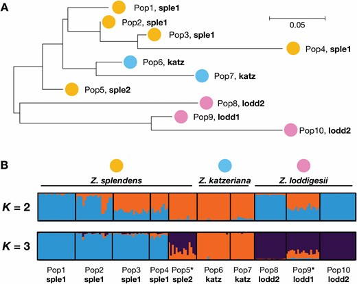
Genetic structure among ten populations of the three examined species: Zamia splendens, Z. katzeriana and Z. loddigesii. A, Graphical representation of the FST values among populations, as constructed in MEGA X (Kumar et al., 2018). The population labels (Pop1–10) and colour labels (Z. splendens in yellow; Z. katzeriana in blue; Z. loddigesii in pink) are accompanied by their group label assigned in the approximate Bayesian analysis. B, Most optimum clustering K = 3 and K = 2 clustering estimated in STRUCTURE (Pritchard et al., 2010). Asterisks indicate two populations that showed patterns of admixture.

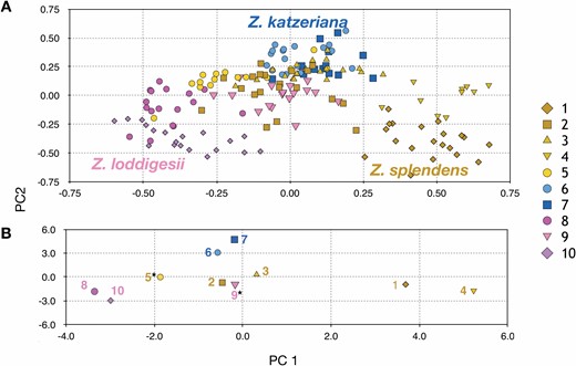
Principal component (PC) plots showing the genetic variation among individuals (A) and among populations (B) of three Zamia species: Z. splendens (yellow, Pop1–5), Z. katzeriana (blue, Pop6–7) and Z. loddigesii (pink, Pop8–10).

The most optimal clustering estimated in STRUCTURE determined by the delta-K method was K = 3 (Fig. 3B, Supporting Information, Fig. S2), each cluster representing one species, but with an extended admixture in pop5 and pop9. Pop5 (Z. splendens) contains alleles more closely related to Z. katzeriana admixed with Z. loddigesii; pop9 (Z. loddigesii) contains alleles of Z. loddigesii admixed with Z. katzeriana and pop5 (Z. splendens). Other clusters showed a relatively low delta-K (Supporting Information, Fig. S2B), with K = 9 and K = 6 being the second and third highest values, respectively, but these clusters are not informative about population grouping. K = 2 had the fourth highest delta-K value, but it complements the interpretation of the clustering K = 3, and we included it in Figure 3B. In combination, the empirical FST values and the STRUCTURE clustering (Fig. 3) distinguished five population groups: sple1 (pops1–4 = ‘pure’ Z. splendens), sple2 (pop5 = Z. splendens admixed), katz (pops6–7 = Z. katzeriana), lodd1 (pop9 Z. loddigesii admixed) and lodd2 (pops 8 and 10 = ‘pure’ Z. loddigesii).
Gene flow and demographic history
Using the private allele method implemented in Genepop, the number of migrants per generation (Nm) was estimated to be <1 in all interspecific comparisons, suggesting no admixture in the long-term (Supporting Information, Table S10). The only case of Nm > 1 was between pop2 and pop3 (1.2628), both populations belonging to Z. splendens. Likewise, MIGRATE-N suggested that historical gene flow among the ten populations was low, Nm ranging from 0.26 to 1.26, and only three pairwise comparisons (among Z. splendens populations) showed values >1 (Supporting Information, Table S11). BayesAss shows a different pattern. This method estimates the proportion of individuals in a population that might have experienced events of allele introgression, and this value was relatively high in one case (=0.2088; in other words, 20.88% of individuals) (Table 3), suggesting patterns of recent introgression of alleles from pop9 (Z. loddigesii) to pop5 (Z. splendens). The Bayesian method implemented in NEWHYBRIDS allowed us to test whether the possible hybrids between pop9 (Z. loddigesii) and pop5 (Z. splendens) were F1, F2 or backcrossed individuals with their neighbouring populations. In this analysis, most individuals in all the evaluated populations were recognized as ‘pure’, with probabilities >0.5 (Supporting Information, Fig. S3). No F1 hybrids were found in either population, but one individual from pop9 (Z. loddigesii) was found likely to be a F2 with a plant from pop5 (Z. splendens) (probability >0.5) (Supporting Information, Fig. S3).
Proportion of migrants in each population (and standard deviation in parentheses) as estimated in BayesAss (Wilson & Rannala, 2003). The highest value (=0.2088) suggests recent gene flow between pop5 (Zamia splendens) and pop9 (Z. loddigesii). Bold values indicate values >0.2.
| From/To | sple | katz | lodd | ||||||||
|---|---|---|---|---|---|---|---|---|---|---|---|
| Pop1 | Pop2 | Pop3 | Pop4 | Pop5 | Pop6 | Pop7 | Pop8 | Pop9 | Pop10 | ||
| sple | Pop1 | 0.8978 | 0.0118 | 0.0113 | 0.0111 | 0.0112 | 0.0111 | 0.0112 | 0.0114 | 0.0117 | 0.0115 |
| (0.0278) | (0.0113) | (0.0109) | (0.0108) | (0.0107) | (0.0108) | (0.0109) | (0.0110) | (0.0113) | (0.0111) | ||
| Pop2 | 0.0115 | 0.8862 | 0.0112 | 0.0112 | 0.0110 | 0.0112 | 0.0111 | 0.0113 | 0.0241 | 0.0112 | |
| (0.0110) | (0.0299) | (0.0107) | (0.0109) | (0.0107) | (0.0109) | (0.0108) | (0.0110) | (0.0179) | (0.0110) | ||
| Pop3 | 0.0113 | 0.0143 | 0.8952 | 0.0111 | 0.0111 | 0.0112 | 0.0112 | 0.0112 | 0.0119 | 0.0114 | |
| (0.0111) | (0.0135) | (0.0286) | (0.0107) | (0.0106) | (0.0110) | (0.0107) | (0.0108) | (0.0115) | (0.0109) | ||
| Pop4 | 0.0221 | 0.0189 | 0.0171 | 0.6832 | 0.0168 | 0.0167 | 0.0164 | 0.0182 | 0.1739 | 0.0167 | |
| (0.0201) | (0.0179) | (0.0163) | (0.0157) | (0.0159) | (0.0159) | (0.0154) | (0.0175) | (0.0378) | (0.0160) | ||
| Pop5 | 0.0131 | 0.0138 | 0.0134 | 0.0133 | 0.6815 | 0.0133 | 0.0132 | 0.0138 | 0.2088 | 0.0157 | |
| (0.0125) | (0.0133) | (0.0129) | (0.0127) | (0.0214) | (0.0127) | (0.0128) | (0.0132) | (0.0369) | (0.0149) | ||
| katz | Pop6 | 0.0123 | 0.0236 | 0.0134 | 0.0121 | 0.0121 | 0.7156 | 0.0255 | 0.0139 | 0.1596 | 0.0119 |
| (0.0119) | (0.0250) | (0.0128) | (0.0118) | (0.0115) | (0.0808) | (0.0194) | (0.0131) | (0.0768) | (0.0115) | ||
| Pop7 | 0.0145 | 0.0149 | 0.0145 | 0.0145 | 0.0144 | 0.0148 | 0.8678 | 0.0146 | 0.0154 | 0.0147 | |
| (0.0140) | (0.0143) | (0.0139) | (0.0138) | (0.0136) | (0.0143) | (0.0336) | (0.0140) | (0.0144) | (0.0140) | ||
| lodd | Pop8 | 0.0122 | 0.0123 | 0.0123 | 0.0122 | 0.0125 | 0.0123 | 0.0122 | 0.8875 | 0.0138 | 0.0126 |
| (0.0117) | (0.0117) | (0.0119) | (0.0118) | (0.0120) | (0.0117) | (0.0119) | (0.0300) | (0.0133) | (0.0121) | ||
| Pop9 | 0.0121 | 0.0118 | 0.0119 | 0.0119 | 0.0120 | 0.0119 | 0.0118 | 0.0119 | 0.8698 | 0.0349 | |
| (0.0117) | (0.0114) | (0.0115) | (0.0115) | (0.0116) | (0.0114) | (0.0115) | (0.0114) | (0.0317) | (0.0212) | ||
| Pop10 | 0.0115 | 0.0115 | 0.0115 | 0.0116 | 0.0115 | 0.0116 | 0.0116 | 0.0116 | 0.0122 | 0.8956 | |
| (0.0111) | (0.0110) | (0.0110) | (0.0111) | (0.0109) | (0.0112) | (0.0112) | (0.0110) | (0.0116) | (0.0282) | ||
Among the ten models of demographic history reconstruction (Supporting Information, Fig. S1), model Sce7 was found to be the most probable (Fig. 5A). This model choice was determined by comparing the modelled datasets with the observed data through direct and logistic regressions (Fig. 5B, C); the two main principal components showed that the posterior values in this model were close to the observed data (Fig. 5D). In this model, all parameters reached good convergence, as shown in Figure S4 (Supporting Information). In this model, the ‘pure’ Z. splendens (sple1; effective population size Ns1 = 19 400) is the earliest diverging, and the ‘pure’ Z. loddigesii (lodd2, Nl2 = 7880) diverged at time t3 = 6140 generations ago. Zamia katzeriana (katz, Nk = 8080) diverged from Z. splendens at time t2 = 4240 generations ago. A second group of Z. loddigesii (lodd1, Nl1 = 6920) diverged from ‘pure’ Z. loddigesii at t1 = 2270 generations ago and admixed with a group of Z. splendens (sple2, Ns2 = 4910) at ta = 1800 generations. Detailed information on the parameter estimations is shown in Table S12 (Supporting Information).
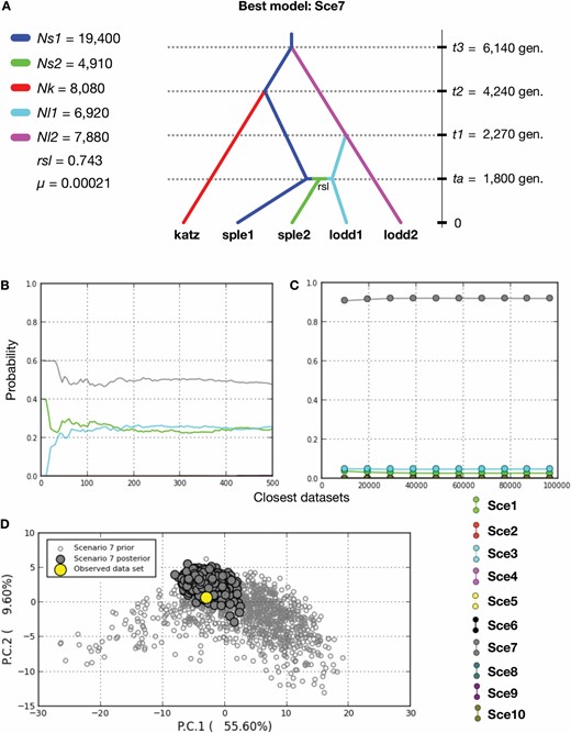
Approximate Bayesian computation model to reconstruct the demographic history and relationships among five groups representing three Zamia species. A, The best of the ten compared models and median values of estimated parameters. Population groups correspond to those obtained in STRUCTURE analyses as shown in Figure 3. Time parameters are given in number of generations and µ is rate in mutations per allele per generation. Detailed information of parameter estimations is shown in Table S12 (Supporting Information). Model Sce7 was found as the most likely model among the competitors in the direct linear (B) and logistic regressions (C). D, The certainty of the model is supported since the posterior values are close to the observed values.

Morphological trait variation
The analyses of morphological variation helped in distinguishing how the traits differ among species (Supporting Information, Fig. S5), among population groups (Fig. 6; Supporting Information, Table S13) and among populations (Fig. S6, Supporting Information, Table S5). The two population groups of Z. loddigesii have significantly more leaflets (Fig. 6B), shorter petioles (Fig. 6C), narrower basal, median and apical leaflets (Fig. 6H–J), a shorter distance between leaflets (Fig. 6K) and narrower leaflet articulations (Fig. 6L) than Z. splendens and Z. katzeriana. Zamia katzeriana can be distinguished from the two groups of Z. splendens by having shorter median leaflets (Fig. 6F) and narrower median and apical leaflets (Fig. 6I, J); the basal leaflets are also narrower, although the differentiation in this trait is not statistically significant (Fig. 6H).
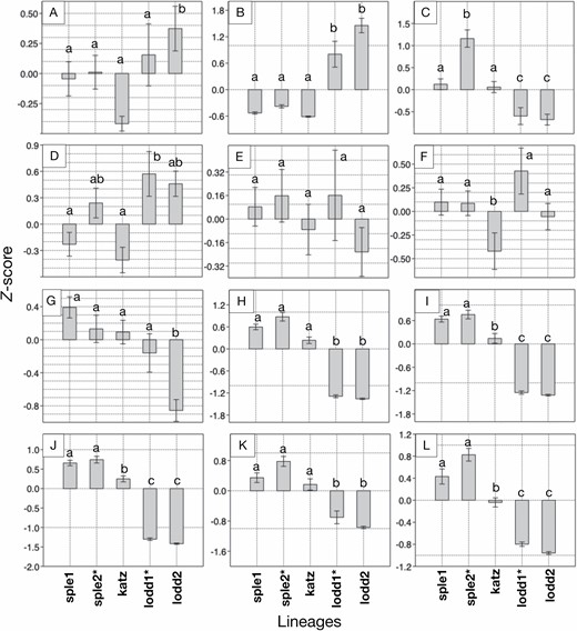
Morphological variation among five analysed population groups of three Zamia species: sple 1 (‘pure’ Z. splendens), sple2 (admixed Z. splendens), katz (Z. katzeriana), lodd1 (admixed loddigesii) and lodd2 (‘pure’ Z. loddigesii). Asterisks indicate the two groups with patterns of admixture. Different lowercase letters above bars indicate significantly differentiated species in the pairwise ANOVA differentiation test. Plots A–L correspond to traits listed in Table 4: A, Number of leaves; B, number of leaflets; C, length of petiole; D, length of rachis; E, length of basal leaflet; F, length of median leaflet; G, length of apical leaflet; H, width of basal leaflet; I, width of median leaflet; J, width of apical leaflet; K, distance between leaflets and L, width of leaflet articulation.

Morphometric traits (designated A–L) analysed in this study and pairwise differentiation between species. Differentiation was tested by calculating the Welch’s F ANOVA value. Abbreviation: sple = Zamia splendens; katz = Z. katzeriana; lodd = Z. loddigesii. Significance: *P < 0.05; **P < 0.01; P < 0.001 (significant differences in bold)
| Abbreviation | Trait | sple vs katz | katz vs lodd | sple vs lodd |
|---|---|---|---|---|
| A | Number of leaves | 3.59 | 13.45*** | 3.309 |
| B | Number of leaflets | 8.979** | 101.3*** | 250.9*** |
| C | Length of petiole | 1.809 | 19.13*** | 33.76*** |
| D | Length of rachis | 1.687 | 21.25*** | 11.95*** |
| E | Length of basal leaflet | 0.6375 | 0.05427 | 1.489 |
| F | Length of median leaflet | 5.393* | 4.996* | 0.02469 |
| G | Length of apical leaflet | 1.458 | 16.19*** | 35.52*** |
| H | Width of basal leaflet | 11.59*** | 468.3*** | 501*** |
| I | Width of median leaflet | 15.58*** | 204.3*** | 500.9*** |
| J | Width of apical leaflet | 15.24*** | 662.8*** | 679.2*** |
| K | Distance between leaflets | 1.772 | 64.26*** | 81.19*** |
| L | Width of leaflet articulation | 7.672** | 150.1*** | 87.5*** |
When focusing on the two groups that showed admixture patterns, we found that the admixed Z. loddigesii group (lodd1) has a significantly lower number of leaves (Fig. 6A) and a longer rachis (Fig. 6G) than the ‘pure’ Z. loddigesii group and is thus more similar to Z. splendens. Likewise, the admixed group of Z. splendens has significantly longer rachis than the ‘pure’ group (Fig. 6D), thus being more similar to Z. loddigesii. We interpret these patterns as possible signals that the length of rachides and the number of leaves, particularly, have been affected by the events of admixture between the admixed groups of Z. splendens (sple2) and Z. loddigesii (lodd1).
In the interspecific pairwise differentiation, Z. splendens is significantly different from Z. katzeriana in six of the 12 morphological traits and is different from Z. loddigesii in ten traits. Zamia katzeriana is different from Z. loddigesii in 11 traits (Table 4). The number of leaflets, the width of basal, median and apical leaflets and the width of leaflet articulations were traits that are significantly differentiated in the three pairwise comparisons between species, suggesting these traits as important for a successful diagnosis. The length of the basal leaflets was the only trait that was not significantly different in any pairwise comparison, and it should not be considered as diagnostic character among these species. Figures S5 and S6 (Supporting Information) show the trait variation across species and populations, respectively, and Table S7 (Supporting Information) shows each pairwise Tukey’s Q values of differentiation at the inter-population level.
The LDA summarized the total variation among the species into two axes (Fig. 7), explaining 93.64 and 3.26%, respectively. The LDA plots of the inter-group variation (Fig. 7) and interspecific variation (Supporting Information, Fig. S7) shows that the two groups of Z. loddigesii can be easily distinguished from the other two species in terms of overall morphological variation, whereas there is an extensive overlap of overall variation between Z. splendens and Z. katzeriana. In the confusion matrix obtained from the LDA, we confirmed that in all populations, the highest number of individuals can be classified as their corresponding groups (Table 5). In the confusion matrix considering the three species as proxies, all populations of Z. splendens and Z. katzeriana contain individuals that might be confused as members of the other species (Supporting Information, Table S14). There are no individuals of Z. splendens or Z. katzeriana that might be confused with Z. loddigesii and no individuals of Z. loddigesii that might be confused with the other two species. However, despite the overlap of morphological variation between Z. splendens and Z. katzeriana, the square-Mahalanobis distances among the three species were found to be significantly high in all cases, supporting morphometric separation among species (Supporting Information, Table S15).
Classification of individuals from ten populations into the five groups of Zamia species analysed, as estimated in the linear discriminant analysis. Bold values highlight the higher numbers of plants of each population classified into one of the three species
| Species—Population | Classified as sple1 (Z. splendens) | Classified as sple2 (Z. splendens) | Classified as katz (Z. katzeriana) | Classified as lodd1 (Z. loddigesii) | Classified as lodd2 (Z. loddigesii) |
|---|---|---|---|---|---|
| Z. splendens—Pop1 | 8 | 6 | 5 | 0 | 0 |
| Z. splendens—Pop2 | 12 | 5 | 1 | 0 | 0 |
| Z. splendens—Pop3 | 9 | 0 | 6 | 0 | 0 |
| Z. splendens—Pop4 | 14 | 1 | 1 | 0 | 0 |
| Z. splendens—Pop5 | 5 | 12 | 1 | 0 | 0 |
| Z. katzeriana—Pop6 | 2 | 0 | 15 | 0 | 0 |
| Z. katzeriana—Pop7 | 2 | 2 | 8 | 0 | 0 |
| Z. loddigesii—Pop8 | 0 | 0 | 0 | 1 | 14 |
| Z. loddigesii—Pop9 | 0 | 0 | 0 | 9 | 3 |
| Z. loddigesii—Pop10 | 0 | 0 | 0 | 10 | 10 |
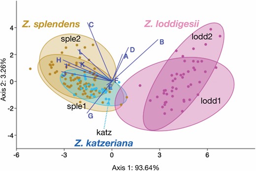
Linear discriminant plot that shows the morphological variation in five groups representing the three analysed Zamia species. Two axes representing 93.64% and 3.26% of the total variation. Biplots A–L correspond to the morphological traits listed in Table 4.

Current and past ecological niche models
Thirty-five, 165 and four occurrence points were obtained for Z. splendens, Z. loddigesii and Z. katzeriana, respectively. The PCA of environmental variation among the ten populations showed that the main principal component (PC) (explaining 96.8% of the total variation) is mainly loaded by variables associated with precipitation seasonality (bio13, bio16, bio19) (Fig. 2C). Populations of Z. splendens occur at areas with more seasonal precipitation, except pop5, which is found in environments more similar to those of pop7 (Z. katzeriana) and Z. loddigesii (pop9 and pop10). These four populations (pop5, 7, 9 and 10) are neighbours occurring in the southern portion of the distribution ranges of the three species (Fig. 2B).
The ENMs of Z. splendens and Z. loddigesii showed high predictive power and did not overfit the data (areas under the curve of ENMs were 0.985 for Z. splendens and 0.942 for Z. loddigesii). Soil type, precipitation of the coldest quarter (bio19) and precipitation seasonality (bio15) were the variables that most contributed to the ENM of Z. splendens (Supporting Information, Table S4). Temperature seasonality (bio4), temperature annual range (bio7) and precipitation of the wettest quarter (bio16) were the variables that most contributed to the ENM of Z. loddigesii (Supporting Information, Table S4). In both species, the niche breadth of the present models was higher than the LGM models, suggesting a niche expansion since the LGM (Fig. 8). The high probabilities of the current niche suitability of Z. loddigesii and Z. splendens are mostly restricted to their actual distribution ranges (Fig. 8A, B), such that the current niche of Z. splendens is mostly restricted to the eastern Isthmus of Tehuantepec, and the niche of Z. loddigesii occurs from south-eastern to north-eastern Mexico. In the LGM (c. 22 kya), the highest probabilities for both species are mostly found on the eastern side of the Isthmus, such that the niche of Z. loddigesii did not exist in north-eastern Mexico (Fig. 8C–F), and the niche of Z. splendens was restricted to narrow areas. This result might indicate two possibilities for Z. splendens: (1) the group maintained its niche in microhabitats that were not detected in the ENMs given the relatively low (30 arc s or 2.5 arc min) resolution of the environmental layers; or (2) the niche has shifted from LGM, such that the current environment where populations occur do not represent the ancestral niche. By observing the niche transition from LGM to present (Fig. 8), it can be observed that the niche of Z. loddigesii has moved from south to north. This pattern suggests that, during its expansion, Z. loddigesii might have tracked the common niche of Zamia spp., and it is likely to have co-occurred in localities with Z. splendens where there might have been chances for secondary contact.
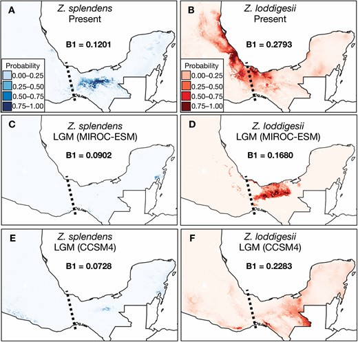
Ecological niche models (ENMs) of Zamia splendens and Z. loddigesii. B1 inverse concentration indexes of niche breadth are annotated. The darker colours indicate higher probabilities of niche suitability. A, B, The geographical distribution of the niche suitability in the present time is estimated based on the variation of nine non-correlated bioclimatic variables. The dotted lines indicate the Isthmus of Tehuantepec. The ENMs were projected onto the bioclimatic variables of the Last Glacial Maximum (LGM), according to the Model for Interdisciplinary Research on Climate East System Model (MIROC-ESM) (C, D) and the Community Climate System Model v.4 (CCSM4) model (E, F). The resulting models suggest that the niches of both species were not present in north-eastern Mexico during the LGM.

Correlations among variables
Genetic distances (phi-values) among populations showed no significant correlation with geographical distances (r = 0.1751; P = 0.2499), elevational differentiation (r = 0.24759; P = 0.1010) or overall environmental dissimilarity (r = 0.19325; P = 0.20341). However, there was a significant correlation between genetic distances and multivariate morphological trait variation among populations (r = 0.3013; P = 0.0442), suggesting that morphological variation among closely related Zamia spp. might have a genetic background. Two morphological traits (number of leaflets and the length of median leaflet) separately showed significant correlations with genetic distances (Table 6). However, all morphological traits (combined and separately) showed high and significant correlations with geographical distances (Table 6). Morphological trait variation did not show significant correlations with elevational differentiation or environmental dissimilarity.
Correlations between morphological traits and geographical and environmental variables. Correlations with genetic differentiation (A), geographical distances (B), elevational differentiation (C) and overall environmental dissimilarity (D). Significant values (in bold) (P < 0.05)
| A, Correlations with phi-values among populations | B, Correlations with geographical distances | C, Correlations with elevational differentiation | D, Correlations with environmental dissimilarity | |||||
|---|---|---|---|---|---|---|---|---|
| r | P | r | P | r | P | r | P | |
| Overall | 0.3013 | 0.0442 | 0.87084 | 7.544E−15 | −0.0707 | 0.6442 | −0.095762 | 0.53148 |
| A: Number of leaves | 0.1235 | 0.4186 | 0.31128 | 0.0374 | −0.1505 | 0.3236 | −0.2368 | 0.11731 |
| B: Number of leaflets | 0.4426 | 0.0023 | 0.7180 | 2.81E−08 | 0.0028 | 0.9851 | −0.078993 | 0.606 |
| C: Length of petiole | −0.2651 | 0.0783 | 0.4396 | 0.0025 | −0.0589 | 0.7005 | −0.11439 | 0.45432 |
| D: Length of rachis | 0.0325 | 0.8320 | 0.5687 | 4.58E−05 | 0.1461 | 0.3380 | 0.18172 | 0.23221 |
| E: Length of basal leaflet | −0.1023 | 0.5034 | 0.3510 | 0.0180 | 0.0796 | 0.6029 | 0.020312 | 0.89464 |
| F: Length of median leaflet | −0.3111 | 0.0374 | 0.3306 | 0.0265 | 0.0656 | 0.6683 | 0.030307 | 0.84334 |
| G: Length of apical leaflet | −0.0259 | 0.8656 | 0.6431 | 1.89E−06 | −0.1938 | 0.2020 | −0.21039 | 0.16538 |
| H: Width of basal leaflet | 0.2147 | 0.1566 | 0.6656 | 6.05E−07 | −0.0220 | 0.8854 | −0.028539 | 0.85237 |
| I: Width of median leaflet | 0.1287 | 0.39947 | 0.6963 | 1.08E−07 | −0.0803 | 0.5999 | −0.059121 | 0.69966 |
| J: Width of apical leaflet | 0.1976 | 0.1930 | 0.7024 | 7.54E−08 | −0.0521 | 0.7336 | −0.036718 | 0.81075 |
| K: Distance between leaflets | −0.1514 | 0.3207 | 0.6378 | 2.44E−06 | −0.1465 | 0.3369 | −0.17999 | 0.23677 |
| L: Width of leaflet articulation | −0.2692 | 0.073642 | 0.6443 | 1.78E−06 | −0.1104 | 0.4701 | −0.13981 | 0.35967 |
DISCUSSION
Zamia katzeriana is not a product of hybridization
Our results suggest that Z. katzeriana is not of hybrid origin, but it rather represents a group derived from the current or ancestral groups of Z. splendens. There is a strong resemblance between Z. splendens and Z. katzeriana, whereas Z. loddigesii is distant in terms of genetic (Fig. 4A) and morphological univariate and multivariate data (Figs 6, 7, Supporting Information, Figs S5–S7, Table S15). The scenario of hybrid origin of Z. katzeriana was modelled in ABC (Scenarios 1 and 2 in Supporting Information, Fig. S1), but they were outperformed by a model that suggests that both Z. katzeriana and Z. loddigesii are both derived from Z. splendens or a direct ancestor of Z. splendens. Zamia katzeriana was estimated to diverge at t2 (4240 generations ago) (Fig. 5). If we consider generation times of ten years, t2 generations would be equivalent to around 42 400 years, before the LGM. A generation time of ten years in Zamia is a conservative, rough, lower estimation that we use because we have observed that species start to produce cones at 3–7 years old in garden conditions (Michael Calonje, pers. comm.; Andrew Vovides, pers. obs.). However, these time estimations should be interpreted carefully because it is uncertain how long generation times for Zamia spp. are at the population level in the wild.
Admixture was detected between Z. splendens and Z. loddigesii (Table 3, Fig. 5). As far as we know, this is the third study, along with the studies by Meerow et al. (2012a) and Tao et al. (2021), that shows estimations suggesting that events of hybridization have occurred in cycad evolution. A question to consider is: as hypothesized by Pérez-Farrera et al. (2016), do the Z. splendens and Z. loddigesii groups that have experienced hybridization resemble the morphology of Z. katzeriana? If this is the case, the pairwise trait differentiation among groups sple2 and lodd1 and katz would not be significant, but it would be significant in respect of sple1 and lodd2. Even so, none of the 12 analysed traits show this expected pattern of differentiation. In contrast, in the hybrid groups (sple2 and lodd1), most traits are not significantly differentiated from their ‘pure’ counterparts; the only two exceptions are that sple2 plants have longer petioles than sple1 (Fig. 6C), lodd1 has shorter apical leaflets than lodd2 (Fig. 6G). Thus, with this evidence, we can confirm that the groups that experienced admixture between Z. splendens and Z. loddigesii do not show morphological similarity with Z. katzeriana, and therefore our results support the idea that the intermediate morphological variation of Z. katzeriana is not due to a hybridization origin as previously thought (Pérez-Farrera et al., 2016).
The idea of the hybrid origin of Z. katzeriana was proposed based on the intermediate morphological and anatomical trait variation that Z. katzeriana has between Z. splendens and Z. loddigesii (Pérez-Farrera et al., 2016). Our analyses at the interspecific and inter-group levels confirm that there is, indeed, an overall intermediate morphological variation among species, as observed in the LDA plots (Fig. 7, Supporting Information, Fig. S6); also, six traits show intermediate differentiation that is significantly differentiated from both Z. splendens and Z. loddigesii (Table 4, Supporting Information, Fig. S5). However, the results clarify that morphological intermediateness of Z. katzeriana with respect to two closely related taxa can be explained by other means rather than hybridization. The environmental factors (and the elevation variable) can be discarded as possible factors influencing the intermediate morphological variation in Z. katzeriana, since we have not detected any significant correlation between the morphological variation and the environmental conditions of the localities where the populations occur (Table 6). Likewise, the PCA plot of environmental variation indicates that populations in the southern portion of the distribution range are similar among species, making it difficult to distinguish a pattern of variation. Also, isolation-by-distance was not supported by genetic data, since correlation between genetic and geographical distances is low (r = 0.1751; P = 0.2499), and an explanation for this is that the geographical ranges of the species overlap and there is no geographical structure, which may influence the linear correlations. On the other hand, we found a significant correlation between the morphological trait variation and the genetic distances among populations (r = 0.3013; P = 0.0442), which in turn, is aligned with the evidence that all the 12 morphological traits separately (and in combination) show significant correlations with linear geographical distances (Table 6). These results suggest that the intermediate variation of Z. katzeriana has a genetic background and the morphological differentiation depicts a pattern that can be explained by isolation-by-distance. Why isolation-by-distance is supported by morphological data but not by genetic data remains uncertain, but a possibility is that microsatellite markers show a different mutation rate that varies among species, given that species might be subjected to different demographic dynamics, as reflected in their distinct effective population sizes (Fig. 5). A phylogenetic approach using DNA sequences or single nucleotide polymorphisms that consider all the Zamia spp. from the study region might be able to detect patterns of morphological variation in relation with the genetic and historical background of the species.
Hybridization between Zamia splendens and Z. loddigesii
The most optimal STRUCTURE clustering at K = 3 (Fig. 3B) distinguishes that pop5 (Z. splendens) and pop9 (Z. loddigesii) are admixed populations. Pop5 includes the orange and purple clusters, and this pattern apparently suggests that pop5 was admixed with both Z. katzeriana and Z. loddigesii. We detected gene flow between pop5 and pop9 (Table 3, Fig. 5), but we found no evidence of gene flow from Z. katzeriana populations to pop5 with the private alleles method (Supporting Information, Table S10) or the Bayesian methods of MIGRATE-N (Table S11 in the Supporting Information), BayesAss (Table 3) and NEWHYBRIDS (Supporting Information, Fig. S3A). Therefore, our interpretation in K = 3 is that the orange cluster represents a group of alleles shared by Z. splendens and Z. katzeriana due to a simple ancestor–descendant relationship. The clustering at K = 2 (Fig. 3B; Supporting Information, Fig. S2) is concordant with this interpretation because pop5 shares the orange cluster with Z. katzeriana, and pops3 and 4 also occur extensively in the orange cluster. Thus, in K = 3, pop9 partially contains the orange cluster not due to an admixture with Z. katzeriana but with Z. splendens (pop5).
BayesAss estimated that a high proportion (> 20%) of individuals in pop5 (Z. splendens, sple2) have experienced allele introgression from pop9 (Z. loddigesii, lodd1) in the last few generations (Table 3). However, NEWHYBRIDS was not able to detect any F1 or backcrossed individuals, and only one individual from pop9 was detected as a possible F2 (Supporting Information, Fig. S3). Also, six individuals from pop5 and seven individuals from pop9 have low probabilities of being non-‘pure’ (Supporting Information, Fig. S3). We interpret these results that introgression existed, but it was not so recent as just a few generations. Ancestral polymorphisms might be an alternative explanation for the shared alleles between pop5 and pop9. However, the fact that these shared alleles are not present in other populations of Z. splendens or Z. loddigesii makes this alternative explanation unlikely.
ABC favours the hypothesis that admixture occurred, but the timing was not recent (Fig. 5). The most probable model needed a timing of a median value of ta = 1800 generations ago to reach convergence. Also, both the private alleles method and MIGRATE-N suggested that the levels of historical gene flow among populations were less than one migrant per generation (Supporting Information, Table S11). Thus, our results may indicate that gene flow has occurred, but it has been scarce and not recurrent. Although BayesAss and NEWHYBRIDS have detected some alleles as introgressed, it is likely that the effect of genetic drift through many generations has diminished their occurrence in the populations. These results might indicate that extrinsic reproductive barriers (e.g. geographical isolation), rather than intrinsic ones (i.e. mating incompatibility, reduced fitness of hybrids), have kept the species in isolation (Nagasawa et al., 2021).
As explained in the Introduction, Z. splendens and Z. loddigesii are placed in separate sister clades in the phylogenetic tree by Calonje et al. (2019). Zamia splendens is phylogenetically closer to other species from primary and secondary rainforests of central Chiapas, Mexico (e.g. Z. cremnophila and Z. purpurea), whereas Z. loddigesii is closer to species with wide distributions in arid, open environments, such as Z. prasina, Z. spartea and Z. furfuracea. Thus, because our ABC model suggests that Z. splendens is ancestor to Z. loddigesii, it is possible that Z. splendens and its close species are relicts that conserve an ancestral humid niche in narrow areas in the Neogene floristic refugia described by Wendt (1989). The niche of Z. splendens in the present and the LGM (c. 22 kya) is mostly restricted to the eastern of Isthmus of Tehuantepec, which is a valley that consists of dry environments that Z. splendens are allies might have not been likely to explore, restricting their dispersal to the western side of the Isthmus, as suggested for other cycads in Mexico (Gutiérrez-Ortega et al., 2020). In contrast, the species of the clade that contains Z. loddigesii evolved broader niches that allowed them to achieve wider distribution ranges (Fig. 8), and the Isthmus was not a barrier to their dispersal. The current and past ENM reconstructions of Z. loddigesii support this idea. In the LGM, the niche of Z. loddigesii was restricted to the south and south-eastern portion of the analysed area (Fig. 8C–F), and the niche suitability in north-eastern Mexico (Sierra Madre Oriental) was non-existent. This suggests that Z. loddigesii reached a broader niche recently, and its dispersal occurred from south-eastern to north-eastern Mexico just after the LGM. ABC suggested that the admixture between Z. loddigesii and Z. splendens was around ta = 1800 generations ago. If we assume generations of ten years, 18 000 years ago would coincide with this possible timing of dispersal. It is likely that during its niche expansion, Z. loddigesii might have been capable to explore new environments where it met Z. splendens in central Chiapas. This might be the main reason why Z. loddigesii is also sympatric with other Zamia spp., such as Z. furfuracea and Z. cremnophila.
Implications for taxonomy and conservation
This research reaffirms that Z. katzeriana is a well-delimited species. It is closely related to Z. splendens in terms of overall morphology, as depicted in the LDA plots (Fig. 7; Supporting Information, Fig. S7). However, only a few individuals can be confused in terms of morphometry when considering such an overall variation (Table 5, Supporting Information, Table S14). Indeed, the separation between Z. splendens and Z. katzeriana occurred > 4200 generations ago (Fig. 5), and the species have sorted morphological differentiation in some of the most important diagnostic characters (i.e. number of leaflets, length of median leaflets, width of basal, median and apical leaflets and width of leaflet articulation) (Table 4), making the two species diagnosable by those characters, in addition to the shiny green colour of leaves that clearly distinguish Z. splendens (hence its Latin name) from Z. katzeriana. The anatomical differences between the two species was also demonstrated in Pérez-Farrera et al. (2016). Thus, our results oppose the suggestion proposed in Nicolalde-Morejón et al. (2008), in which the synonymy of the two taxa was confirmed but not tested. We conclude that Z. katzeriana and Z. splendens are not taxonomic synonyms.
This study also brings important implications for conservation. Using microsatellite data, we produced information on the genetic diversity for three species considered threatened in Mexican legislation (SEMARNAT, 2010). Zamia loddigesii appears as a threatened species (category ‘A’) in NOM-059-SEMARNAT-2010, whereas Z. splendens and Z. katzeriana appear as Endangered (category ‘P’). Likewise, Z. katzeriana and Z. loddigesii appear as Endangered (EN) and Near Threatened species, respectively, in the Red List of the IUCN (Chemnick & Gregory, 2010; Pérez-Farrera & Vovides, 2022). The three species have relatively moderate levels of expected and observed heterozygosity (c. 0.3 to c. 0.6) that are similar to those estimated in other Zamia spp. from Florida (USA) and the Caribbean Islands (Meerow et al., 2012a; Salas-Leiva et al., 2017; Griffith et al., 2022) and Mexico (Favian-Vega et al., 2022). However, none of the examined populations showed dramatically low levels of expected or observed heterozygosity, as was the case for the Mexican species Zamia inermis Vovides, J.D.Rees & Vázq.Torres (Iglesias-Andreu et al., 2017) (c. 0.1 to c. 0.3). Thus, we consider that the populations of Z. splendens, Z. katzeriana and Z. loddigesii are stable, and selective illegal collecting of individuals might not be threatening the populations. In our fieldwork, we observed that Z. loddigesii seems to be able to colonize disturbed areas, but that might not be the case of Z. splendens and Z. katzeriana. Several populations of Z. splendens have been reported (Fig. 2B), but Z. katzeriana is only known from two localities in Chiapas, in areas severely affected by land change due to coffee plantations. Even in the period 1986 to 2000, > 400 000 ha of forest were lost in the El Ocote Biosphere Reserve (Flamenco-Sandoval, Martínez Ramos & Masera, 2007). Thus, conservation in situ and ex situ for Z. katzeriana, in particular, is urgent.
CONCLUSIONS
This study helps clarifying how demographic and historical factors have shaped species delimitation in Zamia. Also, although hybridization is a common topic of discussion in horticulture, here, we provided first discussion on the consequences of hybridization in cycad evolution. We conclude that morphological intermediateness seems to be a common pattern among closely related cycad species, but this alone is insufficient to claim speciation via hybridization. Thus, to date, there is no convincing evidence on the existence of speciation via hybridization in cycads.
SUPPORTING INFORMATION
Additional supporting information may be found in the online version of this article on the publisher’s website.
Figure S1. Approximate Bayesian models [Scenarios (Sce) 1–10] of demographic history of population groups of the three Zamia species evaluated in DIYABC (Cornuet et al., 2014). Sce7 (thick panel margins) was found as the most probable among the competitor models.
Figure S2. Genetic clustering estimated in STRUCTURE (Pritchard et al., 2010). A, Clustering assuming 2 to 10 populations (K = 2–10). Number of iterations (out of 10) that showed similar clustering is indicated. B, Most optimum clustering was determined with the Delta K estimation, according to Evanno et al. (2005). C, Mean of estimated Ln probability of data across K = 1–10.
Figure S3. Clustering results obtained from the analyses in NEWHYBRIDS (Anderson and Thompson, 2002) to test whether the possible hybrids detected in population 5 (Z. splendens) or population 9 (Z. loddigesii) are F1, F2 or backcrossed (Bc) individuals. The asterisk indicates the individual that might be an F2 individual.
Figure S4. Estimations of parameters of approximate Bayesian models of demographic history of three Zamia populations evaluated in DIYABC.
Figure S5. Morphological variation among the three analysed Zamia species: Z. splendens (sple), Z. katzeriana (katz) and Z. loddigesii (lodd). Different lowercase letters above bars indicate significantly differentiated species in the pairwise ANOVA differentiation test. Plots A–L correspond to traits listed in Table 4 and Table S3: A, number of leaves; B, number of leaflets; C, length of petiole; D, length of rachis; E, length of basal leaflet; F, length of median leaflet; G, length of apical leaflet; H, width of basal leaflet; I, width of median leaflet; J, width of apical leaflet; K, distance between leaflets and L, width of leaflet articulation.
Figure S6. Morphological variation among the examined populations (Pop1–10) of three Zamia species: Z. splendens, Z. katzeriana, Z. loddigesii. Traits A–L correspond to those indicated in Table 4 and Table S3.
Figure S7. Morphological variation in three analysed Zamia species. Linear discriminant analysis plot that shows the dispersion of samples of three examined Zamia species along to axes. Biplots A–L correspond to the morphological traits listed in Table 4 and Table S3.
Table S1. Microsatellite loci used in this study
Table S2. Priors used in the approximate Bayesian computation. To facilitate convergence, the following assumptions were imposed: t3 >= t2; t3 >= t1; t3 >= ta; t2 >= t1; t2 >= ta; t1 >= ta; Ns1 >= Ns2; Nl2 >= Nl1; Ns1 >= Nk; Nl2 >= Nk
Table S3. List of morphological traits analysed in this study
Table S4. List of bioclimatic layers used in the Ecological Niche Model constructions and the environmental differentiation analyses. Percentage contribution and permutation importance of variables in the Ecological Niche Model construction of the two examined species are annotated. Bold values indicate the three values with the highest percent contribution for each species’ ENM
Table S5. Matrices of pairwise morphological differentiation among populations. Tukey’s Q among populations (below diagonal) and P values (above diagonal). Matrices A to L correspond to the morphological traits in Table 4 and Table S3. Matrix M corresponds to squared-Mahalanobis distances considering all traits combined
Table S6. Pairwise Fst values among populations (below diagonal) and pairwise phi-values of genetic differentiation among populations (below diagonal); all phi-values are significant (P < 0.001). Abbreviations: sple = Z. splendens; katz = Z. katzeriana; lodd = Z. loddigesii
Table S7. Pairwise environmental differentiation among populations. A, Linear geographic distances (in km); B, altitudinal differentiation (Euclidian distances) and C, multivariate environmental dissimilarity (considering the nine bioclimatic variables combined)
Table S8. Tests of data integrity. A, Results obtained in MicroChecker v.2.2.3 (Van Oosterhout et al., 2004). Loci showing an excess of homozygotes in populations are indicated with “Excess”. NS = no significantly exceeded homozygosity. Populations 1, 4 and 8 could not be tested due to low sampling size. B, Significance of chi-square tests for Hardy–Weinberg equilibrium of loci on populations. *P < 0.05, **P < 0.01; P < 0.001; NS, not significant; Mono, monomorphic locus
Table S9. Analysis of molecular variance (AMOVA) among the examined populations and species
Table S10. Number of migrants (Nm) among populations estimated with the private alleles method. Values >1 are in bold
Table S11. Theta values (Θ) and levels of historical gene flow among the ten analysed populations as estimated in MIGRATE-N (Beerli and Felsenstein, 1999, 2001). The number of migrants per generation was estimated via ΘaMa→b = 4Nma. Nm values above 1 are annotated in bold text
Table S12. Estimation of demographic parameters in approximate Bayesian computation. Parameters were estimated based in the 1% of the datasets closest to the observed data of the most probable model in the analysis
Table S13. Matrices of pairwise morphological differentiation among population groups. Tukey’s Q among populations (below diagonal) and P values (above diagonal). Matrices A to L correspond to the morphological traits in Table 4 and Table S3. Matrix M corresponds to squared-Mahalanobis distances considering all traits combined
Table S14. Classification of individuals into the three Zamia species analysed, as estimated in the linear discriminant analysis. Bold values highlight the higher numbers of plants of each population classified into one of the three species
Table S15. Morphological squared-Mahalanobis distances among analysed Zamia species (below diagonal) and P values (above diagonals)
ACKNOWLEDGEMENTS
Thanks to three anonymous reviewers for giving us comments that were useful to improve our research and manuscript. Thanks to anonymous donors to the Montgomery Botanical Center for financial support to MAPF. MAPF also thanks Christopher Davidson and Sharon Christoph for financial support in the project ‘Floristic diversity and evolutionary ecology of endangered species in protected natural Areas in Chiapas, Mexico’. APV acknowledges SEP-CONACYT for financing the project number CB-2011-01-169468. Samples and specimens were collected under permit SGPA/DGVS/12737 from SEMARNAT, Mexico.
CONFLICT OF INTEREST
The authors declare no conflict of interest.
DATA AVAILABILITY
The data underlying this article are available in Figshare at https://doi.org/10.6084/m9.figshare.21561789.v1.