Abstract
Open sets are central to mathematics, especially analysis and topology, in ways few notions are. In most, if not all, computational approaches to mathematics, open sets are only studied indirectly via their ‘codes’ or ‘representations’. In this paper, we study how hard it is to compute, given an arbitrary open set of reals, the most common representation, i.e. a countable set of open intervals. We work in Kleene’s higher order computability theory, in particular its equivalent lambda calculus formulation due to Platek. We establish many computational equivalences between on one hand the ‘structure’ functional that converts open sets to the aforementioned representation, and on the other hand functionals arising from mainstream mathematics, like basic properties of semi-continuous functions, the Urysohn lemma and the Tietze extension theorem. We also compare these functionals with known operations on regulated and bounded variation functions, and the Lebesgue measure restricted to closed sets. We obtain a number of natural computational equivalences for the latter involving theorems from mainstream mathematics.
1 Introduction
1.1 Motivation and overview
First of all, computability theory is a discipline in the intersection of theoretical computer science and mathematical logic where the fundamental question is as follows:
If X and Y are real numbers, Turing’s ‘machine’ model ([84]) is the standard approach, i.e. ‘computation’ is interpreted in the sense of Turing machines. To formalize computation involving (total) abstract objects, like functions on the real numbers or well-orderings of the reals, Kleene introduced his S1–S9 computation schemes in [44]. In Section 5, we introduce a version1 of the lambda calculus involving fixed point operators that exactly captures S1–S9 and accommodates partial objects, with a brief introduction in Section 1.2.1. Henceforth, any reference to computability is to be understood in Kleene’s framework and (if relevant) the extension to partial objects from Section 5. For those not intimate with S1–S9, we hasten to add that many of our positive results, i.e. of the form |$X$| is computable from |$Y$|, are actually of the form |$X$| is computable from |$Y$| via a term of Gödel’s |$T$| of low complexity. However, these are only examples and we have no structural results at this point.
Secondly, the notion of open (and closed) set is central to mathematics, especially topology and analysis, in ways few mathematical definitions are. Historically, the concept of open set dates back to Baire’s doctoral thesis ([5]), while Dedekind already studied such notions twenty years earlier; the associated paper [17] was only published much later ([56]). Now, for various reasons, the computational study of open sets usually takes place indirectly, namely via representations or codes for open sets, as discussed in detail in Remark 1.4. In this light, it is a natural question how hard it is to compute such representations in terms of open sets. In this paper, we study this question for the well-known representation of open sets of reals as countable unions of open intervals. We identify a large number of operations that have the same computational complexity and compare the latter with known operations from [65, 66] stemming from mainstream mathematics, including the Lebesgue measure restricted to closed sets. We discuss some open problems related the previous in Section 4.
Thirdly, in more detail, the following functional constitutes the central object of study in this paper. We note that open and closed sets are given by characteristic functions (see Section 1.2.3), well-known from e.g. probability theory.
The |$\varOmega _{C}$|-functional is defined exactly when the input |$X\subset 2^{\mathbb N}$| is a closed set, in which case |$\varOmega _{C}(X)=0$| if |$X=\emptyset $| and |$\varOmega _{C}(X)=1$| if |$X\ne \emptyset $|.
We have shown in [61] that |$\varOmega _{C}$| is hard2 to compute. In Section 2, we shall introduce the |$\varOmega _{C}$|-cluster, a collection of functionals that are computationally equivalent (see Def. 2.2) to |$\varOmega _{C}$|, assuming Kleene’s quantifier |$\exists ^{2}$| from Section 1.2.2. We identify a large number of elements of the |$\varOmega _{C}$|-cluster, many stemming from mainstream mathematics, like properties of semi-continuous functions. The following list contains some representative members of the |$\varOmega _{C}$|-cluster studied in Section 2.
A partial functional |$\varPhi :({\mathbb R}\rightarrow{\mathbb R})\rightarrow{\mathbb R}$| such that for open |$O\subset [0,1]$|, |$\varPhi (O)$| is a code for |$O$| (see [78, Section II.5.6] for the latter).
A partial functional |$\varPhi :({\mathbb R}\rightarrow{\mathbb R})\rightarrow{\mathbb R}$| such that for any upper semi-continuous |$f:[0,1]\rightarrow{\mathbb R}$| and |$p, q\in{\mathbb Q}\cap [0,1]$|, |$\varPhi (f)=\sup _{x\in [p, q]}f(x)$|.
A partial functional |$\varPhi :({\mathbb R}\rightarrow{\mathbb R})\rightarrow \{0,1\}$| such that for any upper semi-continuous |$f:[0,1]\rightarrow{\mathbb R}$|, |$\varPhi (f)=0$| if and only |$f$| is continuous on |$[0,1]$|.
Witnessing functionals for Urysohn lemma and Tietze extension theorem.
Interestingly, computing suprema or deciding continuity for arbitrary functions requires Kleene’s quantifier |$\exists ^{3}$|. We obtain similar equivalences for the Lebesgue measure restricted to closed sets in Section 3.5. In this study, we shall always assume Kleene’s |$\exists ^{2}$| from Section 1.2.2 to be given; we motivate this assumption by the observation that we mainly study discontinuous functions on the reals, from which |$\exists ^{2}$| is readily obtained via Grilliot’s trick ([31, 46]).
Fourth, we shall compare the properties of |$\varOmega _{C}$| with the |$\varOmega _{b}$|-functional, where the latter was studied in [65, 66]. We note that we may replace |$2^{\mathbb N}$| with |$[0,1]$| or |${\mathbb N}^{\mathbb N}$| in Def. 1.2 without consequence. At this moment, we do not know whether |$\varOmega _{C}$| and |$\varOmega _{b}$| are computationally equivalent, as reflected in Problem 4.1 below.
The |$\varOmega _{b}$|-functional is defined exactly when the input |$X\subset 2^{\mathbb N}$| has at most one element, in which case |$\varOmega _{b}(X)=0$| if |$X=\emptyset $| and |$\varOmega _{b}(X)=1$| if |$X\ne \emptyset $|.
Assuming Kleene’s |$\exists ^{2}$| from Section 1.2.2, the functional |$\varOmega _{b}$| is computationally equivalent to the functional |$\varOmega $| defined as follows (see [66, Lemma 3.3.5])
The functional |$\varOmega (X)$| is defined if |$|X| \leq 1$| and outputs the element of |$X$| when |$|X| = 1$| and the constant |$0^{1}$| when |$X = \emptyset $|.
We have previously studied the |$\varOmega _{b}$|-cluster (called ‘|$\varOmega $|-cluster’ in [66]), which is the collection of functionals that are computationally equivalent (see Def. 2.2) to |$\varOmega _{b}$|, assuming |$\exists ^{2}$|. A number of natural operations on bounded variation and regulated functions are in the |$\varOmega _{b}$|-cluster. We shall exhibit notable differences and similarities between the |$\varOmega _{b}$|- and |$\varOmega _{C}$|-cluster. One important similarity is that |$\varOmega _{C}$| is lame by Theorem 3.3, i.e. the combination |$\varOmega _{C}+\exists ^{2}$| computes the same real numbers as Kleene’s |$\exists ^{2}$|. By Theorem 3.5, there are even no total functionals ‘in between’ |$\varOmega _{C}$| and |$\varOmega _{b}$| from the computational point of view. Nonetheless, we identify a number of natural partial functionals in Section 3.3 that are intermediate in this way. An important difference between |$\varOmega _{b}$| and |$\varOmega _{C}$| is that they witness basic properties of two different function classes, namely the bounded variation and semi-continuous functions, although there is overlap between the latter.
On a conceptual note, |$\varOmega _{C}$| and |$\varOmega _{b}$| are examples of what we call a structure functional, i.e. a functional that does not turn up as a result of some construction in mainstream mathematics, but which is nonetheless useful for calibrating the computational complexity of those that do, like the functionals associated to Urysohn’s lemma and the Tietze extension theorem.
Figure 1 shows some connections between |$\varOmega _{C}$|, |$\varOmega _{b}$| and related functionals, like the Lebesgue measure |${\pmb{\lambda }}_{C}$| restricted to closed sets. Moreover, Baire and (weak) Cantor realizers are witnessing functionals for the Baire category theorem and the uncountability of |${\mathbb R}$|, while a Cantor intersection functional is a witnessing functional for the Cantor intersection theorem (see Def. 1.12 and 3.8). All functionals are computable in |$\exists ^{3}$| and strictly weaker than the latter.
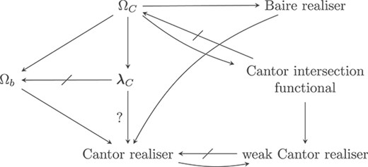
Some relations among our functionals.

Finally, open sets are studied indirectly via ‘codes’ or ‘representations’ in computational approaches to mathematics. The following historical remark provides an overview of some such computational approaches to open sets.
A set is open if it contains a neighbourhood around each of its points, and an open set can be represented as a countable union of such neighbourhoods in separable spaces, a result going back to Cantor. The latter and similar representations are used in various ‘computational’ approaches to mathematics, as follows.
For instance, the neighbourhood around a point of an open set is often assumed to be given together with this point (see e.g. [7, p. 69]). This is captured by our representation R2 studied in [61, §7] and below. Alternatively, open sets are simply represented as countable unions—called ‘codes’ in [78, Section II.5.6], ‘names’ in [87, §1.3.4], ‘witnesses’ in [88] and ‘presentations’ in [23]—of basic open neighbourhoods. A related notion is locatedness which means the (continuous) distance function |$d(a, A):=\inf _{b\in A}d(a, b)$| exists for the set |$A\subset{\mathbb R}$| (see [7, p. 82], [28] or [86, p. 258]), and numerous sufficient conditions are known ([28]).
The representation of open sets as countable unions has the advantage that one can (effectively) switch between codes for open sets and codes for continuous functions (see e.g. [78, Section II.7.1]). As shown in [45, 61, 67], computing a code for a continuous function, say on Cantor or Baire space or the unit interval, is rather easy, while computing a code for an open set is rather hard, in the sense of Footnote 2.
1.2 Preliminaries and definitions
We briefly introduce Kleene’s higher order computability theory in Section 1.2.1. We introduce some essential axioms (Section 1.2.2) and definitions (Section 1.2.3). A full introduction may be found in e.g. [64, §2] or [50].
Since Kleene’s computability theory borrows heavily from type theory, we shall often use common notations from the latter; for instance, the natural numbers are type |$0$| objects, denoted |$n^{0}$| or |$n\in{\mathbb N}$|. Similarly, elements of Baire space are type |$1$| objects, denoted |$f\in{\mathbb N}^{{\mathbb N}}$| or |$f^{1}$|. Mappings from Baire space |${\mathbb N}^{{\mathbb N}}$| to |${\mathbb N}$| are denoted |$Y:{\mathbb N}^{{\mathbb N}}\rightarrow{\mathbb N}$| or |$Y^{2}$|. An overview of such notations can be found in e.g. [50, 66].
1.2.1 Kleene’s computability theory
Our main results are in computability theory and we make our notion of ‘computability’ precise as follows.
(I) We adopt |$\textsf{ZFC}$|, i.e. Zermelo–Fraenkel set theory with the Axiom of Choice, as the official metatheory for all results, unless explicitly stated otherwise.
(II) We adopt Kleene’s notion of higher order computation as given by his nine clauses S1–S9 (see [50, Ch. 5] or [44]) as our official notion of ‘computable’ involving total objects.3
We mention that S1–S8 are rather basic and merely introduce a kind of higher order primitive recursion with higher order parameters. The real power comes from S9, which essentially hard-codes the recursion theorem for S1–S9-computability in an ad hoc way. By contrast, the recursion theorem for Turing machines is derived from first principles in [79].
On a historical note, it is part of the folklore of computability theory that many have tried (and failed) to formulate models of computation for objects of all finite types and in which one derives the recursion theorem in a natural way. For this reason, Kleene ultimately introduced S1–S9, which were initially criticized for their aforementioned ad hoc nature, but eventually received general acceptance. Now, the authors have introduced a new computational model based on the lambda calculus in [66] with the following properties:
S1–S8 is included while the ‘ad hoc’ scheme S9 is replaced by more natural (least) fixed point operators,
the new model exactly captures S1–S9 computability for total objects,
the new model accommodates ‘computing with partial objects’,
the new model is more modular than S1–S9 in that sub-models are readily obtained by leaving out certain fixed point operators.
As noted in Section 1.1, the lambda calculus from [66] contains a technical error, which was recently discovered by John Longley. We discuss a fix in Section 5. This involves essentially replacing the calculus from [66] with one essentially from Platek [70] and recovering the computation tree characterization from [66] as Theorem 5.8.
Next, we mention the distinction between ‘normal’ and ‘non-normal’ functionals based on the following definition from [50, §5.4]. We only use |$\exists ^{n}$| for |$n=2,3$|, as defined in Section 1.2.2.
For |$n\geq 2$|, a functional of type |$n$| is called normal if it computes Kleene’s quantifier |$\exists ^{n}$| following S1–S9, and non-normal otherwise.
It is a historical fact that higher order computability theory, based on Kleene’s S1–S9, has focused primarily on the world of normal functionals; this observation can be found [50, §5.4] and can be explained by the (then) relative scarcity of interesting non-normal functionals, like the fan functional, originally due to Kreisel (see [68] for historical details). The authors have recently identified interesting non-normal functionals, namely those that compute the objects claimed to exist by
covering theorems due to Heine–Borel, Vitali and Lindelöf ([60]),
local-global principles like Pincherle’s theorem ([60]),
weak fragments of the Axiom of (countable) Choice ([62]),
the Jordan decomposition theorem and related results ([65, 66]),
This paper continues the study of non-normal functionals that originate from basic properties of closed sets and semi-continuous functions.
Finally, the first example of a non-computable non-normal functional, Kreisel’s (aka Tait’s) fan functional (see [68]), is rather tame: it is computable in |$\exists ^{2}$|. By contrast, the functionals based on the previous list, including the operation (2.7) from Section 1.1, are computable in |$\exists ^{3}$| but not computable in any |$\textsf{S}_{k}^{2}$|, where the latter decides |$\varPi _{k}^{1}$|-formulas (see Section 1.2.2 for details).
1.2.2 Some comprehension functionals
In Turing-style computability theory, computational hardness is measured in terms of where the oracle set fits in the well-known comprehension hierarchy. For this reason, we introduce some functionals related to higher order comprehension in this section. We are mostly dealing with conventional comprehension here, i.e. only parameters over |${\mathbb N}$| and |${\mathbb N}^{{\mathbb N}}$| are allowed in formula classes like |$\varPi _{k}^{1}$| and |$\varSigma _{k}^{1}$|.
First of all, Kleene’s quantifier |$\exists ^{2}: {\mathbb N}^{{\mathbb N}}\rightarrow \{0,1\} $| is the unique functional satisfying
Clearly, |$\exists ^{2}$| is discontinuous at |$f=11\dots $| in the usual epsilon-delta sense. In fact, given a discontinuous function on |${\mathbb N}^{{\mathbb N}}$| or |${\mathbb R}$|, Grilliot’s trick computes |$\exists ^{2}$| from the former, via a rather low-level term of Gödel’s |$T$| (see [46, §3]). Moreover, |$\exists ^{2}$| computes Feferman’s |$\mu ^{2}$| defined for any |$f^{1}$| as follows:
Hilbert and Bernays formalize considerable swaths of mathematics using only |$\mu ^{2}$| (with that name) in [39, Supplement IV].
Secondly, the Suslin functional |$\textsf{S}^{2}:{\mathbb N}^{{\mathbb N}}\rightarrow \{0,1\}$| (see [4, 46]) is the unique functional satisfying the following, for any |$f^{1}$|:
By definition, the Suslin functional |${\textsf{S}}^{2}$| can decide whether a |$\varSigma _{1}^{1}$|-formula as in the left-hand side of (1.3) is true or false. We similarly define the functional |${\textsf{S}}_{k}^{2}$| which decides the truth or falsity of |$\varSigma _{k}^{1}$|-formulas, given in their Kleene normal form (see e.g. [78, Section IV.1.4]). The Feferman–Sieg operators |$\nu _{n}$| from [15, p. 129] are essentially |${\textsf{S}}_{n}^{2}$| strengthened to return a witness (if existent) to the |$\varSigma _{n}^{1}$|-formula at hand.
Thirdly, Kleene’s quantifier |$\exists ^{3}: ({\mathbb N}^{{\mathbb N}}\rightarrow{\mathbb N})\rightarrow \{0,1\} $| is the functional satisfying:
Hilbert and Bernays introduce functionals in e.g. [39, Supplement IV, p. 479] that readily compute |$\exists ^{3}$|.
In conclusion, the functionals in Figure 1 from Section 1.1 are computable in |$\exists ^{3}$| but not in any type 2 functional, which includes |${\textsf{S}}_{k}^{2}$| from Section 1.2.2 (see [61, 63, 65] for proofs). Many non-normal functionals exhibit the same ‘computational hardness’ and we merely view this as support for the development of a separate scale for classifying non-normal functionals.
1.2.3 Some definitions
We introduce some definitions needed in the below, mostly stemming from mainstream mathematics. We note that subsets of |${\mathbb R}$| are given by their characteristic functions (Definition 1.6), where the latter are common in measure and probability theory.
First of all, we use usual definition of (open) set, where |$B(x, r)$| is the open ball with radius |$r>0$| centred at |$x\in{\mathbb R}$|. Note that ‘RM’ stands for ‘Reverse Mathematics’ in the final items.
Subsets |$A$| of |$ {\mathbb R}$| are given by their characteristic function |$F_{A}:{\mathbb R}\rightarrow \{0,1\}$|, i.e. we write |$x\in A$| for |$ F_{A}(x)=1$| for all |$x\in{\mathbb R}$|.
We write ‘|$A\subset B$|’ if we have |$F_{A}(x)\leq F_{B}(x)$| for all |$x\in{\mathbb R}$|.
A subset |$O\subset{\mathbb R}$| is open in case |$x\in O$| implies that there is |$k\in{\mathbb N}$| such that |$B(x, \frac{1}{2^{k}})\subset O$|.
A subset |$C\subset{\mathbb R}$| is closed if the complement |${\mathbb R}\setminus C$| is open.
A subset |$O\subset{\mathbb R}$| is R2-open in case there is |$Y:{\mathbb R}\rightarrow{\mathbb R}$| such that |$x\in O$| implies |$Y(x)>0\wedge B(x, Y(x))\subset O$| and |$Y(x)=0\rightarrow x\not \in O$|, for any |$x\in{\mathbb R}$|.
A subset |$C\subset{\mathbb R}$| is R2-closed if the complement |${\mathbb R}\setminus C$| is R2-open.
A subset |$O\subset{\mathbb R}$| is RM-open if there are sequences |$(a_{n})_{n\in{\mathbb N}}, (b_{n})_{n\in{\mathbb N}}$| of reals such that |$O=\cup _{n\in{\mathbb N}}(a_{n}, b_{n})$|.
A subset |$C\subset{\mathbb R}$| is RM-closed if the complement |${\mathbb R}\setminus C$| is RM-open.
No computational data/additional representation is assumed in our definition of open set. As established in [65, 66, 76], one readily comes across closed sets in basic real analysis (Fourier series) that come with no additional representation. The function |$Y:{\mathbb R}\rightarrow{\mathbb R}$| is called an R2-representation for the R2-open set |$O$| and the sequences |$(a_{n})_{n\in{\mathbb N}}, (b_{n})_{n\in{\mathbb N}}$| are called an R4-representation (see [61]) or RM-code for the RM-open set |$O$|.
Secondly, the following sets are often crucial in proofs in real analysis.
The sets |$C_{f}$| and |$D_{f}$|, respectively, gather the points where |$f:{\mathbb R}\rightarrow{\mathbb R}$| is continuous and discontinuous.
One problem with |$C_{f}, D_{f}$| is that ‘|$x\in C_{f}$|’ involves quantifiers over |${\mathbb R}$|. In general, deciding whether a given |${\mathbb R}\rightarrow{\mathbb R}$|-function is continuous at a given real is as hard as |$\exists ^{3}$| from Section 1.2.2. For these reasons, the sets |$C_{f}, D_{f}$| do exist in general, but are not computable in e.g. |$\exists ^{2}$|. For quasi-continuous and semi-continuous functions, these sets are definable in |$\exists ^{2}$| by [66, §2] or [77, Theorem 2.4], a fact we use often.
Thirdly, to avoid the problem sketched in the previous formula, one can additionally assume the existence of the oscillation function |${\textsf{osc}}_{f}:{\mathbb R}\rightarrow{\mathbb R}$| as in Def. 1.8. The formula ‘|$x\in C_{f}$|’ is then equivalent to the arithmetical formula |${\textsf{osc}}_{f}(x)=_{{\mathbb R}}0$|.
For any |$f:{\mathbb R}\rightarrow{\mathbb R}$|, the associated oscillation functions are defined as follows: |${\textsf{osc}}_{f}([a,b]):= \sup _{{x\in [a,b]}}f(x)-\inf _{{x\in [a,b]}}f(x)$| and |${\textsf{osc}}_{f}(x):=\lim _{k \rightarrow \infty } {\textsf{osc}}_{f}(B(x, \frac{1}{2^{k}}) ).$|
We note that Riemann, Hankel and Ascoli already study the notion of oscillation in the context of Riemann integration ([3, 33, 72]).
Fourth, we shall study the following notions, many of which are well-known and hark back to the days of Baire, Darboux, Hankel and Volterra ([5, 6, 16, 33, 34, 85]).
For |$f:[0,1]\rightarrow{\mathbb R}$|, we have the following definitions:
|$f$| is upper semi-continuous at |$x_{0}\in [0,1]$| if |$f(x_{0})\geq _{{\mathbb R}}\lim \sup _{x\rightarrow x_{0}} f(x)$|,
|$f$| is lower semi-continuous at |$x_{0}\in [0,1]$| if |$f(x_{0})\leq _{{\mathbb R}}\lim \inf _{x\rightarrow x_{0}} f(x)$|,
|$f$| is quasi-continuous at |$x_{0}\in [0, 1]$| if for |$ \epsilon> 0$| and an open neighbourhood |$U$| of |$x_{0}$|, there is a non-empty open |${ G\subset U}$| with |$(\forall x\in G) (|f(x_{0})-f(x)|<\varepsilon )$|.
|$f$| is cliquish at |$x_{0}\in [0, 1]$| if for |$ \epsilon> 0$| and an open neighbourhood |$U$| of |$x_{0}$|, there is a non-empty open |${ G\subset U}$| with |$(\forall y, z\in G) (|f(y)-f(z)|<\varepsilon )$|.
|$f$| is regulated if for every |$x_{0}$| in the domain, the ‘left’ and ‘right’ limit |$f(x_{0}-)=\lim _{x\rightarrow x_{0}-}f(x)$| and |$f(x_{0}+)=\lim _{x\rightarrow x_{0}+}f(x)$| exist.
|$f$| is Baire 0 if it is a continuous function.
|$f$| is Baire |$n+1$| if it is the pointwise limit of a sequence of Baire |$n$| functions.
|$f$| is Baire 1|$^{*}$| if4 there is a sequence of closed sets |$(C_{n})_{n\in{\mathbb N}}$| such that |$[0,1]=\cup _{n\in{\mathbb N}}C_{n}$| and |$f_{\upharpoonright C_{m}}$| is continuous for all |$m\in{\mathbb N}$|.
|$f$| is continuous almost everywhere if it is continuous at all |$x\in [0,1]\setminus E$|, where |$E$| is a measure zero5 set.
|$f$| is pointwise discontinuous if for any |$x\in [0,1]$| and |$\varepsilon>0$|, there is |$y\in [0,1]$| such that |$f$| is continuous at |$y$| and |$|x-y|<\varepsilon $| (Hankel, 1870, [33]).
As to notations, a common abbreviation is ‘usco’ and ‘lsco’ for the first two items. Moreover, if a function has a certain weak continuity property at all reals in |$[0,1]$| (or its intended domain), we say that the function has that property. We shall generally study |${\mathbb R}\rightarrow{\mathbb R}$|-functions but note that ‘usco’ and ‘lsco’ are also well-defined for |$f:[0,1]\rightarrow \overline{{\mathbb R}}$|, where |$\overline{{\mathbb R}}={\mathbb R}\cup \{+\infty , -\infty \}$| involves two special symbols that satisfy |$(\forall x\in{\mathbb R})(-\infty <_{{\mathbb R}} x <_{{\mathbb R}}+\infty )$| by fiat.
We note that cliquish functions are exactly those functions that can be expressed as the sum of two quasi-continuous functions ([11]). Nonetheless, these notions can behave fundamentally different (see e.g. [66, §2.8]).
Fifth, the notion of bounded variation (abbreviated |$BV$|) was first explicitly6 introduced by Jordan around 1881 ([41]) yielding a generalization of Dirichlet’s convergence theorems for Fourier series. Indeed, Dirichlet’s convergence results are restricted to functions that are continuous except at a finite number of points, while functions of bounded variation can have (at most) countable many points of discontinuity, as already studied by Jordan, namely in [41, p. 230]. Nowadays, the total variation of |$f:[a, b]\rightarrow{\mathbb R}$| is defined as follows:
If this quantity exists and is finite, one says that |$f$| has bounded variation on |$[a,b]$|. Now, the notion of bounded variation is defined in [58] without mentioning the supremum in (1.5); see also [12, 13, 48]. Hence, we shall distinguish between the following notions. Jordan seems to use item (1.10) of Definition 1.10 in [41, p. 228-229].
(a) The function |$f:[a,b]\rightarrow{\mathbb R}$| has bounded variation on |$[a,b]$| if there is |$k_{0}\in{\mathbb N}$| such that |$k_{0}\geq \sum _{i=0}^{n-1} |f(x_{i})-f(x_{i+1})|$| for any partition |$x_{0}=a <x_{1}< \dots < x_{n-1}<x_{n}=b $|.
(b) The function |$f:[a,b]\rightarrow{\mathbb R}$| has a variation on |$[a,b]$| if the supremum in (1.5) exists and is finite.
The fundamental theorem about |$BV$|-functions (see e.g. [41, p. 229]) is as follows.
A function |$f: [0, 1] \rightarrow{\mathbb R}$| of bounded variation is the difference of two non-decreasing functions |$g, h:[0,1]\rightarrow{\mathbb R}$|.
Theorem 1.11 has been studied extensively via second-order representations in e.g. [30, 48, 58, 89]. The same holds for constructive analysis by [12, 13, 38, 69], involving different (but related) constructive enrichments. Now, arithmetical comprehension suffices to derive Theorem 1.11 for various kinds of second-order representations of |$BV$|-functions in [48, 58]. By contrast, the results in [63–66] show that the Jordan decomposition theorem is even ‘explosive’: combining with the Suslin |${\textsf{S}}^{2}$| (see Section 1.2.2), one derives the much stronger |${\textsf{S}}_{2}^{2}$|.
Finally, we have previously studied the following functionals in e.g. [61, 65, 66], also found in Figure 1 in Section 1.1.
A Baire realizer is defined for input |$(O_{n})_{n\in{\mathbb N}}$| being a sequence of open and dense sets in |$[0,1]$|; the output is any |$x\in \cap _{n\in{\mathbb N}}O_{n}$|.
A Cantor realizer is defined for input |$(A, Y)$| where |$Y:{\mathbb R}\rightarrow{\mathbb N}$| is injective on |$A\subset [0,1]$|; the output is any real |$x\in [0,1]\setminus A$|.
A weak Cantor realizer is defined for input |$(A, Y)$| where |$Y:{\mathbb R}\rightarrow{\mathbb N}$| is injective on |$A\subset [0,1]$| and satisfies |$(\forall n\in{\mathbb N})(\exists x\in A)(Y(x)=n)$|; the output is any real |$x\in [0,1]\setminus A$|.
2 Populating the |$\varOmega _{C}$|-cluster
2.1 Introduction
In this section, we introduce the |$\varOmega _{C}$|-cluster and establish that many functionals originating from mainstream mathematics belong to this cluster. For instance, many functionals witnessing basic properties of semi-continuous functions turn out to be members of the |$\varOmega _{C}$|-cluster, as well as functionals witnessing the Urysohn lemma and Tietze extension theorem.
First of all, we recall the definition of |$\varOmega _{C}$| from Section 1.1.
The |$\varOmega _{C}$|-functional is defined exactly when the input |$X\subset 2^{\mathbb N}$| is a closed set, in which case |$\varOmega _{C}(X)=0$| if |$X=\emptyset $| and |$\varOmega _{C}(X)=1$| if |$X\ne \emptyset $|.
The |$\varOmega _{C}$|-cluster is now defined as the following equivalence class.
We say that the functional |$\varPhi ^{3}$| belongs to the |$\varOmega _{C}$|-cluster in case
the combination |$\varPhi +\exists ^{2}$| computes |$\varOmega _{C}$|, and
the combination |$\varOmega _{C}+\exists ^{2}$| computes |$\varPhi $|.
We also say that the functionals |$\varPhi $| and |$\varOmega _{C}$| are computationally equivalent given |$\exists ^{2}$|.
Secondly, to avoid complicated definitions and domain restrictions, we will sometimes abuse notation and make statements of the form
The centred statement means that for any functional |$\varPsi _{0}$| satisfying the given specification |$\mathsf{(A)}$|, the combination |$\varPsi _{0}+\exists ^{2}$| computes |$\varOmega _{C}$|, while |$\varOmega _{C}+\exists ^{2}$| computes some functional |$\varPsi _{1}$| satisfying the specification |$\varPsi _{1}$|.
Finally, as to content, this section is structured as follows.
In Section 2.2, we identify a large number of functionals in the |$\varOmega _{C}$|-cluster, grouped in the first and second cluster theorem. These are all generally related to semi-continuity and properties of closed/compact sets.
In Section 2.3, we identify some functionals in or related to the |$\varOmega _{C}$|-cluster that deal with the following (in our opinion) ‘unexpected’ topics:
Regarding the second bullet point, it is known that many basic properties of arbitrary functions on the reals are only decidable given |$\exists ^{3}$|. The crux is of course that we additionally assume an oscillation function to be given in Section 2.3.1. The latter function is always upper semi-continuous, explaining the connection to |$\varOmega _{C}$|.
2.2 The cluster theorems
We establish the first (Theorem 2.3) and second (Theorem 2.5) cluster theorems, identifying a large number of members of the |$\varOmega _{C}$|-cluster. Many of these members are based on mainstream results pertaining to semi-continuous functions and exhibit some robustness. We assume that the functionals |$\varPhi _{1}$|-|$\varPhi _{7}$| in Theorem 2.3 are undefined outside of their (clearly specified) domain of definition to avoid complicated specifications.
The following belong to the |$\varOmega _{C}$|-cluster.
The partial functional |$\varPhi _{0}$| that to a compact subset |$X$| of |${\mathbb N}^{\mathbb N}$| outputs 0 if |$X$| is empty and 1 otherwise.
The partial functional |$\varPhi _{1}$| that to a closed subset |$X$| of |$[0,1]$| outputs 0 if |$X$| is empty and 1 otherwise.
The partial functional |$\varPhi _{2}$| that to an open set |$O \subset [0,1]$| outputs the set of pairs |$\langle p,q\rangle $| of rational numbers such that |$(p,q) \subseteq O$|.
The partial functional |$\varPhi _{2,c}$| that to an open set |$O \subset [0,1]$| outputs the set of pairs |$\langle p,q\rangle $| of rational numbers such that |$[p,q] \subseteq O$|.
The partial functional |$\varPhi _{3}$| that to usco |$f:[0,1]\rightarrow{\mathbb R}$| outputs |$\sup _{x\in [0,1]} f(x)$|.
Any partial functional |$\varPhi _{4}$| that to usco |$f:[0,1]\rightarrow{\mathbb R}$| outputs |$y\in [0,1]$| where |$f$| attains its supremum.
Any selector |$\varPhi _{5}$| for compact |$X\subset 2^{\mathbb N}$|, i.e. |$\varPhi _{5}(X) \in 2^{\mathbb N}$| for all compact |$X$|, and |$\varPhi _{5}(X) \in X$| when |$X \neq \emptyset $|.
Any functional |$\varPhi _{5, c}$| that to closed |$C\subset [0,1]$| and |$k\in{\mathbb N}$|, outputs distinct |$x_{0}, \dots , x_{k}\in C$| if such there are, and |$0$| otherwise.
Any functional |$\varPhi _{6}$| that to a perfect subset of |$[0,1]$| outputs its optimal RM-code, alternatively (and equivalently) decides if a set that is either perfect or empty, is empty or perfect.
The functional |$\varPhi _{7}$| that to a closed subset |$X$| of |$2^{\mathbb N}$| outputs its optimal code.
Zeroth, a closed subset of |$2^{\mathbb N}$|, is a compact subset of |${\mathbb N}^{\mathbb N}$|, so |$\varOmega _{C}$| is a sub-function of |$\varPhi _{0}$| and thus computable in it. For the other direction we use that there is a Turing-computable injection from |${\mathbb N}^{\mathbb N}$| to |$2^{\mathbb N}$| with a partial Turing-computable inverse. Using this, we readily compute |$\varPhi _{0}$| from |$\varOmega _{C}$|
First of all, if |$X \subseteq [0,1]$| is closed, then the set of binary expansions of the elements in |$X$| is a compact subset of |$2^{\mathbb N}$|, so we can use |$\varOmega _{C}$| to decide if |$X$| is non-empty or not. In this way, |$\varOmega _{C}$| computes |$\varPhi _{1}$| and the other direction is trivial. Without loss of generality, we shall often write |$\varOmega _{C}$| for |$\varPhi _{1}$|.
Secondly, if |$O$| is an open subset of |$[0,1]$| and |$r < q$| are rational points in |$[0,1]$|, we can use |$\varPhi _{1}$| to decide if |$[r,q] \subseteq O$| or not. Using |$\exists ^{2}$|, this information yields |$\varPhi _{2}(O)$|. So |$\varPhi _{1}$| computes |$\varPhi _{2}$|, and by the same argument |$\varPhi _{2, c}$|. Conversely, if |$X \subseteq [0,1]$| is closed and |$\varPhi _{2}$| provides us with an RM-code for |$[0,1] \setminus X$|, then |$\exists ^{2}$| can check if this code contains a finite sub-covering of |$[0,1]$| or not, i.e. if |$X$| is empty or not. Thus, |$\varPhi _{2}$| computes |$\varPhi _{1}$|, and so does |$\varPhi _{2, c}$|.
Thirdly, if |$f:[0,1]\rightarrow{\mathbb R}$| is usco, then for any |$r\in{\mathbb Q}$| we have that |$\{x \in [0,1]: f(x) \geq r\}$| is closed. Using this and |$\exists ^{2}$|, |$\varPhi _{1}$| computes the Dedekind cut of |$\sup f$|, i.e. |$\varPhi _{1}$| computes |$\varPhi _{3}$|. If |$X \subseteq 2^{\mathbb N}$| is compact, we consider |$X$| as a closed subset of the (traditional) Cantor set. Then the characteristic function of |$X$| is usco. Using |$\varPhi _{3}$| to find the sup of this function, we can decide if |$X$| is empty or not, thus computing |$\varOmega _{C}(X)$|, i.e. |$\varPhi _{3}$| and |$\varPhi _{4}$| compute |$\varOmega _{C}$|. For the reversal, let |$f:[0,1] \rightarrow{\mathbb R}$| be usco and use |$\varPhi _{3}$| to find |$a = \sup f$|, and define |$X:= \{x: f(x) = a\}$|. Then |$X$| is closed and non-empty, i.e. |$\varPhi _{2}$| yields an RM-code for |$X$|. From this RM-code we can define the least element of |$X$| arithmetically, i.e. using |$\exists ^{2}$|, yielding |$\varPhi _{4}$|.
Fourth, any |$\varPhi _{5}$| clearly computes |$\varOmega _{C}$|, while the other direction proceeds as follows: let |$X\subset 2^{{\mathbb N}}$| be compact and use |$\varOmega _{C}$| to compute the set of basic neighbourhoods in |$2^{\mathbb N}$| disjoint from |$X$|. Use |$\varOmega _{C}$| to decide if |$X$| is non-empty and, if it is, locate the lexicographically least element of |$X$| using the usual interval-halving technique. The proof for |$\varPhi _{5, c}$| proceeds in the same way.
Fifth, |$\varPhi _{6}$| is trivially computable from |$\varOmega _{C}$|; for the other direction it suffices to show that if we can decide between perfect and empty sets, we can also decide if a closed set is empty or not. Thus, let |$X \subseteq [0,1]$| be closed. If |$X \cap{\mathbb Q}\neq \emptyset $|, then |$X \neq \emptyset $|. If |$X$| and |${\mathbb Q}$| are disjoint, then |$X$| is homeomorphic to the set of binary representations for the elements of |$X$|, i.e. |$X$| can be regarded as a closed subset of |$2^{\mathbb N}$|. Using the bijection between |$2^{\mathbb N}$| and |$2^{\mathbb N}\times 2^{{\mathbb N}}$|, we consider the set |$X \times 2^{\mathbb N}$|. This set is perfect if |$X$| is non-empty, and empty otherwise. We can then use |$\varPhi _{6}$| on this set to decide if |$X$| is empty or not. The final item is done in the same way.
Regarding |$\varPhi _{3}$| in Theorem 2.3, it goes without saying that finding suprema for usco functions amounts to the same as finding infima for lsco functions. Moreover, the definition of ‘honest RM-code for an lsco function’ from [24, §5] amounts to assuming that |$(\forall x\in B(a, r))(f(x)\geq q)$| is |$\varSigma _{1}^{0}$| with parameters |$r, q, a\in{\mathbb Q}$|. The latter formula is clearly equivalent to |$q\leq \inf _{x\in B(a, r)}f(x)$|, i.e. the notion of honest code is connected to |$\varPhi _{3}$| from Theorem 2.3.
Next, we establish the second cluster theorem as in Theorem 2.5, for which we first introduce the following definition, an essential part of Ekeland’s variational principle ([21]), well known from analysis.
Clearly, |$\varPhi _{18}$| and |$\varPhi _{19}$| in Theorem 2.5 express Ekeland’s variational principle.
Regarding |$\varPhi _{22}$|, the latter witnesses [57, Theorem 2] which states that a set |$S\subset [0,1]$| is |$\textbf{F}_{\sigma }$| if and only if there is a Baire 1 |$f:[0,1]\rightarrow{\mathbb R}$| such that |$S=\{x\in [0,1]:f(x)\ne 0\}$|. Similarly, |$\varPhi _{23}$| is based on the fact that the Baire 1 sets are exactly those in |$\textbf{F}_{\sigma }\cap \textbf{G}_{\delta }$| (see [73, Theorem 11.6]). Moreover, |$\varPhi _{29}$| computes a Lebesgue number7 for an enumerated covering of open sets.
We (again) assume that the functionals in Theorem 2.5 are undefined outside of their (clearly specified) domain of definition.
The following belong to the |$\varOmega _{C}$|-cluster.
The functional |$\varPhi _{8}$| that to a closed set |$C\subset [0,1]$|, outputs |$\sup C$|.
The functional |$\varPhi _{9}$| that to closed |$C\subset [0,1]$| and continuous |$f:C\rightarrow{\mathbb R}$|, outputs |$\sup _{x\in C} f(x)$|.
The functional |$\varPhi _{10}$| that to closed |$C\subset [0,1]$| and usco |$f:[0,1]\rightarrow{\mathbb R}$|, outputs |$\sup _{x\in C} f(x)$|.
(Urysohn) Any functional |$\varPhi _{11}$| that to closed disjoint |$C_{0}, C_{1}\subset [0,1]$|, outputs continuous |$f:[0,1]\rightarrow{\mathbb R}$| with |$x\in C_{i}\leftrightarrow f(x)=i$| for |$x\in [0,1]$|, |$i\leq 1$|.
(weak Urysohn) Any ‘weak’ functional |$\varPhi _{11, w}$| which is the previous item with ‘continuity’ replaced by ‘Baire 1’ or ‘quasi-continuity’.
(Tietze) Any functional |$\varPhi _{12}$| that to closed |$C\subset [0,1]$| and continuous |$f:C\rightarrow{\mathbb R}$| outputs continuous |$g:[0,1]\rightarrow{\mathbb R}$| such that |$g(x)=f(x)$| for |$x\in C$|.
(Tietze–Haussdorf, [37, 82]) Any functional |$\varPhi _{13}$| that to closed |$C\subset [0,1]$| and lsco |$f:[0,1]\rightarrow{\mathbb R}$| continuous on |$C$| outputs an increasing sequence |$(f_{n})_{n\in{\mathbb N}}$| of continuous functions with pointwise limit |$f$| and |$f=f_{n}$| on |$C$|.
The functional |$\varPhi _{14}$| that for usco |$f:[0,1]\rightarrow{\mathbb R}$| decides whether |$C_{f}=\emptyset $|.
The functional |$\varPhi _{15}$| that for usco |$f:[0,1]\rightarrow{\mathbb R}$| decides whether |$f\in BV$| and outputs |$V_{0}^{1}(f)$| if so.
Any functional |$\varPhi _{16}$| that to usco |$f:[0,1]\rightarrow{\mathbb R}$| outputs a decreasing sequence of continuous functions |$(f_{n})_{n\in{\mathbb N}}$| with pointwise limit |$f$|.
Any functional |$\varPhi _{17}$| that to usco |$f:[0,1]\rightarrow{\mathbb R}$|, outputs a sequence of continuous functions |$(f_{n})_{n\in{\mathbb N}}$| with infimum |$f$| (Dilworth lemma, [18, Lem. 4.1]).
(Ekeland) Any functional |$\varPhi _{18}$| that to lsco |$f:[0,1]\rightarrow{\mathbb R}$| and |$\varepsilon>0$| outputs an |$\varepsilon $|-critical point |$x\in [0,1]$|.
(Ekeland) Any functional |$\varPhi _{19}$| that to lsco |$f:[0,1]\rightarrow{\mathbb R}$| outputs |$x\in [0,1]$| such that for all |$\varepsilon>0$|, |$x$| is |$\varepsilon $|-critical.
Any functional |$\varPhi _{20}$| that to usco |$f:[0,1]\rightarrow{\mathbb R}$| outputs an (honest) RM-code |$\varPhi $| that equals |$f$| on |$[0,1]$|.
(Hahn–Katětov–Tong insertion theorem [32, 42, 83]) The functional |$\varPhi _{21}$| that to usco |$f:[0,1]\rightarrow{\mathbb R}$| and lsco |$g: [0,1]\rightarrow{\mathbb R}$| with |$(\forall x\in [0,1])(f(x)\leq g(x))$| outputs continuous |$h:[0,1]\rightarrow{\mathbb R}$| with |$(\forall x\in [0,1])(f(x)\leq h(x)\leq g(x))$|.
Any functional |$\varPhi _{22}$| that to a sequence |$(C_{n})_{n\in{\mathbb N}}$| of closed sets in |$[0,1]$| outputs Baire 1 |$f:[0,1]\rightarrow{\mathbb R}$| and its representation such that |$\cup _{n\in{\mathbb N}}C_{n}=\{x\in [0,1]:f(x)\ne 0\}$|.
Any functional |$\varPhi _{23}$| that to closed |$C\subset [0,1]$| outputs increasing |$f:{\mathbb R}\rightarrow{\mathbb R}$| such that |$f^{\prime}$| is continuous and |$C=\{ x\in [0,1]: f^{\prime}(x)=0 \}$| ([73, Ex. 1.P]).
The functional |$\varPhi _{24}$| that to usco |$f:[0,1]\rightarrow{\mathbb R}$| outputs the associated ‘rising sun function’ |$f_{\odot }$|, i.e. the minimal decreasing |$g:[0,1]\rightarrow{\mathbb R}$| such that |$g\geq f$|.
The functional |$\varPhi _{25}$| that for usco |$f:[0,1]\rightarrow \overline{{\mathbb R}}$| decides whether |$f$| is bounded above by some |$N\in{\mathbb N}$|.
The functional |$\varPhi _{26}$| that for usco |$f:[0,1]\rightarrow \overline{{\mathbb R}}$| decides whether |$f$| is Riemann integrable on |$[0,1]$|.
The functional |$\varPhi _{27}$| that for closed |$C\subset [0,1]$| decides whether |$C$| is a closed interval or not.
(Finkelstein [26]) Any functional |$\varPhi _{28}$| that for lsco |$f:[0,1]\rightarrow [0,+\infty )$| outputs continuous |$h:([0,1]\times{\mathbb R})\rightarrow [0, +\infty )$| such that for each |$x\in [0,1]$|, |$\lambda y.h(x, y)$| is integrable and |$f(x)=\int _{-\infty }^{+\infty }h(x, y)dy$|.
Any functional |$\varPhi _{29}$| that to an open covering |$(O_{n})_{n\in{\mathbb N}}$| of |$[0,1]$| outputs a Lebesgue number7 for the covering.
First of all, |$\varPhi _{8}$| can decide whether a closed |$C\subset [0,1]$| is non-empty by checking |$[0<\varPhi _{8}(C\cup \{0\})] \vee [0\in C]$| using |$\exists ^{2}$|. For the reversal, |$\varPhi _{2}$| from the first cluster theorem provides an RM-code and |$\exists ^{2}$| readily yields the supremum by [78, Section IV.2.11]. Clearly, items |$\varPhi _{9}$| and |$\varPhi _{10}$| readily compute |$\varPhi _{8}$| by considering |$f(x):=x$| while the other direction follows using |$\exists ^{2}$| by [78, IV.2.11] and |$\varPhi _{3}$| from the first cluster theorem. For the latter, obtain a code for the closed set and use |$\varPhi _{3}$| on the intervals of the code.
Secondly, the equivalence involving |$\varPhi _{11}$| is proved in [61, Theorem 5.3]. For |$\varPhi _{11, w}$|, it suffices to show that the latter computes |$\varPhi _{1}$|. Hence, let |$X\subset (0,1)$| be closed, put |$C_{1}=X$| and |$C_{0}=\{0\}$| and let |$f_{X}:[0,1]\rightarrow{\mathbb R}$| be the Baire 1 (or quasi-continuous) function provided by |$\varPhi _{11, w}$|. By (the proof of) [67, Theorem 2.9], |$\exists ^{2}$| can compute |$\sup _{x\in [0,1]}f_{X}(x)$|, both for Baire 1 and quasi-continuous functions, and we have |$X=\emptyset \leftrightarrow [1>\sup _{x\in [0,1]}f_{X}(x)]$|, where the right-hand side is decidable using |$\exists ^{2}$|. The Tietze functional |$\varPhi _{12}$| computes the Urysohn functional |$\varPhi _{11}$| as follows: for closed and disjoint |$C_{0}, C_{1}\subset [0,1]$|, define |$C:= C_{0}\cup C_{1}$| and let |$f:C\rightarrow{\mathbb R}$| be |$0$| on |$C_{0}$| and |$1$| on |$C_{1}$|. Now apply the former functional to obtain the latter. To compute |$\varPhi _{12}$|, use |$\varOmega _{C}$| to obtain an RM-code for |$C\subset [0,1]$|. To obtain a code for |$f:C\rightarrow{\mathbb R}$|, the proof of [67, Theorem 2.3], relativizes to the RM-code of |$C$|. With this code in place, the standard second-order proof of the Tietze extension theorem yields an RM-code defined on |$[0,1]$| that equals |$f$| on |$C$|. Clearly, |$\mu ^{2}$| converts this code into a third-order function.
Fifth, to show that |$\varPhi _{4}$| computes |$\varPhi _{18}$| and |$\varPhi _{19}$|, let |$x_{0}\in [0,1]$| be such that |$f(x_{0})=\inf _{x\in [0,1]}f(x)$|, i.e. |$f$| attains its minimum at |$x_{0}$|. Fix |$\varepsilon>0$| and suppose (2.1) is false, i.e. there is |$y\ne x_{0}$| such that |$\varepsilon |y-x_{0}|\leq f(x_{0})-f(y)$|. This implies |$f(x_{0})>f(y)$| and contradicts the minimum property of |$x_{0}$|. Hence, |$x_{0}$| is |$\varepsilon $|-critical for all |$\varepsilon>0$|. Now assume |$\varPhi _{18}$| and let |$(x_{k})_{k\in{\mathbb N}}$| be a sequence in |$[0,1]$| such that |$x_{k}$| satisfies (2.1) for |$\varepsilon =\frac{1}{2^{k}}$|, for any |$k\in{\mathbb N}$|. Let |$(y_{k})$| be a convergent sub-sequence, say with limit |$y\in [0,1]$|, all found using |$\exists ^{2}$|. We now show that |$f(y)=\inf _{x\in [0,1]}f(x)$|, i.e. |$\varPhi _{4}$| is obtained. To this end, suppose there is |$z\in [0,1]$| such that |$f(z)<f(y)$|. Since |$f$| is lsco, there is |$k_{0}\in{\mathbb N}$| such that |$f(z)+\frac{1}{2^{k_{0}}}<f(y_{k})$| for |$k\geq k_{0}$|. Hence, there is |$k\geq k_{0}$|, such that |$\frac{1}{2^{k}}|y_{k}-z| \leq f(y_{k})-f(z)$|. Since |$y_{k}$| is |$\frac{1}{2^{k}}$|-critical, we obtain |$z=y_{k}$|, a contradiction.
Seventh, |$\varPhi _{21}$| computes a realizer for the Urysohn lemma as follows: let |$C_{0}, C_{1}$| be disjoint subsets of |$[0,1]$| and define |$O_{1}:=[0,1]\setminus C_{1}$|. Apply |$\varPhi _{21}$| to |$f(x):= \mathbb{1}_{C_{0}}(x)$| and |$g(x):= \mathbb{1}_{O_{1}}(x)$| and note that the resulting continuous |$h:[0,1]\rightarrow{\mathbb R}$| is such that |$x\in C_{i}\rightarrow h(x)=1-i$| for |$x\in [0,1]$| and |$i\in \{0,1\}$|, i.e. as required for the Urysohn lemma. For the reversal, one observes that the proof of [29, Theorem 1] goes through without modification.
Eight, for a closed set |$C\subset [0,1]$|, |$\varPhi _{22}$| provides a Baire 1 representation of |$\mathbb{1}_{C}$|. By (the proof of) [67, Theorem 2.9], |$\exists ^{2}$| computes the supremum of Baire 1 functions. Hence, we can decide whether |$C$| is non-empty, yielding |$\varOmega _{C}$|. For the other direction, the proof of [73, Theorem 11.6] shows that |$\varPhi _{3}$| computes |$\varPhi _{22}$|. To compute |$\varPhi _{24}$|, we have |$f_{\odot }(x)=\sup _{y\in [x, 1]} f(y)$| for usco |$f$| (see [73, Excercise 1.G]), i.e. |$\varPhi _{3}$| computes the former functional. For the other direction, |$\varPhi _{24}$| allows us to compute |$\sup _{x\in [p, q]}f(x)$| by applying the former to |$F$| defined as follows: |$F(f, x, q):= f(x)$| for |$x\leq q$| and |$f(q)$| otherwise. For fixed |$q$| and usco |$f$|, |$\lambda x.F(f,x, q)$| is also usco. To show that |$\varPhi _{23}$| computes |$\varPhi _{2}$|, in case |$C=\{ x\in [0,1]: g(x)=0 \}$| where |$C$| is closed and |$g$| continuous, one readily computes an RM-code. Indeed, |$\exists ^{2}$| suffices to compute the sup and inf of continuous functions (see [46, §3]). To compute |$\varPhi _{23}$|, let |$C$| be closed and consider |$d(x, C)$|, which is computable in terms of |$\exists ^{2}$| and an RM-code for |$C$|. Since the distance function is continuous, use |$\exists ^{2}$| to define |$f_{C}(x):=\int _{0}^{x}d(y, C)dy$|. Clearly, this function is increasing and satisfies the other conditions for |$\varPhi _{23}$| in light of the fundamental theorem of calculus.
Nineth, regarding |$\varPhi _{25}$| and |$\varPhi _{26}$|, let |$C\subset [0,1]$| be closed and define the usco function |$\mathbb{2}_{C}:[0,1]\rightarrow \overline{{\mathbb R}}$| as follows: |$\mathbb{2}_{C}(x):= +\infty $| in case |$x\in C$| and |$\mathbb{2}_{C}(x)=0$| otherwise. Clearly, |$C=\emptyset \leftrightarrow (\exists N\in{\mathbb N})(\forall x\in [0,1])(\mathbb{2}_{C}(x)\leq N) $|, i.e. |$\varPhi _{25}$| computes |$\varOmega _{C}$|. The same holds for |$\varPhi _{26}$| as Riemann integrability implies boundedness. For the other direction, let |$f:[0,1]\rightarrow \overline{{\mathbb R}}$| be usco and note that this function is finitely bounded above if and only if |$(\exists N\in{\mathbb N})( E_{N}=\emptyset )$| for the closed set |$E_{n}:=\{ x\in [0,1]: f(x)\geq n\}$|. Hence, |$\varPhi _{1}$| computes |$\varPhi _{25}$|. For |$\varPhi _{26}$|, we note that Riemann integrability is equivalent to boundedness plus continuity almost everywhere. The latter property is equivalent to the closed sets |$D_{f, q}$| from (2.2) having measure zero for all |$q\in{\mathbb Q}^{+}$|. Now |$\varPhi _{2}(D_{f, q})$| yields an RM-code for these sets and |$\exists ^{2} $| can decided whether the codes have measure zero. Hence, |$\varPhi _{26}$| is also computable from |$\varOmega _{C}$|.
Tenth, to compute |$\varPhi _{27}$| from |$\varPhi _{8}$|, let |$C\subset [0,1]$| be closed and use |$\varPhi _{8}$| to obtain |$\sup C$| (and |$\inf C$|). In case |$\inf C<_{{\mathbb R}} \sup C$|, the set |$C$| equals the interval |$[\inf C, \sup C]$| if and only if |$(\forall q\in{\mathbb Q}\cap [\inf C, \sup C])(q\in C)$|. Now assume |$\varPhi _{27}$| and consider an open set |$O\subset [0,1]$| where |$C:=[0,1]\setminus O$|; define the closed sets |$L_{q}:= C\cap [0, q]$| and |$R_{q}:= C\cap [q, 1]$| and note that |$O$| is an open interval if and only if |$(\forall q\in{\mathbb Q}\cap O)({{L}}_{q} \text{and}\ R_{q} \text{are intervals} )$|. Hence, |$\varPhi _{27}$| allows us to decide whether an open set |$O\subset [0,1]$| is an interval. Since |$(p, q)\subset O$| if and only if |$(p, q)\cap O$| is an interval, |$\varPhi _{2}$| can be computed, as required.
Eleventh, to compute |$\varPhi _{28}$|, the proof of [26, Theorem 1] guarantees that given lsco |$f:[0,1]\rightarrow [0, +\infty )$|, the function |$h:([0,1]\times{\mathbb R})\rightarrow [0, +\infty )$| is definable (using only |$\exists ^{2}$|) from an increasing sequence |$(f_{n})_{n\in{\mathbb N}}$| of continuous functions with pointwise limit |$f$|; this sequence is obtained from |$\varPhi _{16}$|. The other direction is also immediate from the aforementioned proof.
Finally, the combination |$\varOmega _{C}+\exists ^{2}$| computes an RM-code of an open set, from which |$\exists ^{2}$| readily computes a Lebesgue number as required for |$\varPhi _{29}$|. For the other direction, let |$X \subseteq [0,1]$| be closed and let |$\varPhi _{29}$| be given. We will use |$\exists ^{2}$| and |$\varPhi _{29}$| to decide if |$X$| is empty or not. Let |$\big ((p_{n},q_{n})\big )_{n \in{\mathbb N}}$| be an enumeration of all pairs of rational numbers |$p < q$| in |$ [0,1]$| and let |$O_{n} = (p_{n},q_{n}) \cap [0,1]$| be the associated open covering. Further, if |$[a,b] \subseteq [0,1]$| we write ‘|$x \in [a,b]^{ X}$|’ if |$\frac{x - a}{b-a} \in X$|. Intuitively, |$[a,b]^{X}$| is the range of |$X$| under the affine map from |$[0,1]$| onto |$[a,b]$|.
Now fix |$\delta _{0}:= \varPhi (\lambda n.O_{n})$| and let us construct a new covering |$(O^{\prime}_{n})_{n \in{\mathbb N}}$| from the given one, depending on |$X$| and |$\delta _{0}$|. Our construction will guarantee that each |$O^{\prime}_{n} = O_{n}$| if |$X = \emptyset $| while no |$O^{\prime}_{n}$| will contain an interval of length |$\delta _{0}$| if |$X \neq \emptyset $|. We can then test if |$X$| is empty or not by testing if |$\varPhi (\lambda n.O^{\prime}_{n}) = \delta _{0}$| or not.
For the construction, if |$q_{n} - p_{n} < \delta _{0}$|, we put |$O^{\prime}_{n} = O_{n}$|, which ensures that our new sequence of sets will be a covering of |$[0,1]$|. If |$q_{n} - p_{n} \geq \delta _{0}$|, we let |$k\in{\mathbb N}$| be such that |$\frac{q_{n} - p_{n}}{k} < \delta _{0}$|, and we put |$a_{n,i}: = p_{n} + i(\frac{q_{n} - p_{n}}{k})$| for |$i = 0, \ldots ,k$|. Finally, we define |$O^{\prime}_{n}$| from |$O_{n}$| by removing all elements of the subsets of |$O_{n}$| of the form |$[a_{n,i},a_{n,i+1}]^{X} $| for |$i = 0, \ldots , k-1$|. This new open covering clearly has the properties described in the previous paragraph, and we are done.
Regarding |$\varPhi _{15}$|, we could generalize to regulated functions and output the associated Waterman variation (see [2]). Regarding |$\varPhi _{18}$| and |$\varPhi _{19}$|, we could similarly study the Caristi fixed point theorem based on its second-order development in [25]. Regarding |$\varPhi _{21}$|, we could obtain similar equivalences for the insertion theorems by Dowker and Michael ([20, 54]), following the proofs in [29]. We note that Hahn was the first to prove the above insertion theorem for metric spaces ([32]). Regarding |$\varPhi _{26}$|, we note that the Lebesgue integral is not suitable here. Finally, we could also generalize certain results to Baire 1|$^{*}$| as the latter amounts to the sum of an usco and a lsco function by [53].
2.3 More on the |$\varOmega _{C}$|-cluster
We establish further results related to the |$\varOmega _{C}$|-cluster as follows.
We identify functionals in the |$\varOmega _{C}$|-cluster that decide basic properties of arbitrary functions (Section 2.3.1).
We generalize the notion of modulus of continuity and identify functionals in the |$\varOmega _{C}$|-cluster that output these generalizations (Section 2.3.2).
In Section 2.3.3, we (briefly) study computational equivalences for |$\varOmega _{C}$| (and |$\varOmega $|) assuming functionals stronger than |$\exists ^{2}$|.
Most of the results in Sections 2.3.1–2.3.3 could be included in the cluster theorems of Section 2.2; nonetheless, we believe the former deserve their own section, due to their novelty but also in the interest of clarity of presentation.
2.3.1 Computing with arbitrary functions
To decide basic properties of arbitrary functions |$f:[0,1]\rightarrow{\mathbb R}$|, like boundedness or Riemann integrability, one needs (exactly) Kleene’s |$\exists ^{3}$|. In this section, we show that additionally assuming an oscillation function as input, the decision procedure is more tame, namely |$\varOmega _{C}$|.
The following functionals belong to the |$\varOmega _{C}$|-cluster:
for input any |$f:[0,1]\rightarrow{\mathbb R}$| with oscillation function, decide if |$f$| is continuous or not on |$[0,1]$|.
for input any |$f:[0,1]\rightarrow{\mathbb R}$| with oscillation function, decide if |$f$| is continuous or not, and output |$x\in D_{f}$| in the latter case and a modulus of continuity in the former.
for input any |$f:[0,1]\rightarrow{\mathbb R}$| with oscillation function, decide if |$f$| is in |$BV$| or not on |$[0,1]$|, and output |$V_{0}^{1}(f)$| in the former case.
For the second item, in case |$D_{k}\ne \emptyset $|, the usual interval-halving technique will provide |$x\in D_{k}\subset D_{f}$|. A modulus of continuity for a continuous function is computable in |$\exists ^{2}$| by [45, §4].
For the third item, assume |$\varOmega _{C}$| and consider again the closed set |$D_{k}$| from (2.4). Using |$\varPhi _{5, c}$| from Theorem 2.3, we can decide whether |$D_{k}$| is finite, and if so, enumerate it. Now, assuming |$D_{f}$| is countable and given an enumeration of this set, |$\exists ^{2}$| can compute |$V_{0}^{1}(f)$| (if it exists) as the supremum in (1.5) now runs over |${\mathbb Q}\times{\mathbb N}$|. Hence, we obtain the third centred functional. To show that the third centred functional computes |$\varOmega _{C}$|, note that for a closed set |$C\subset [0,1]$|, one has |$C=\emptyset $| if and only if |$\mathbb{1}_{C}$| is in |$BV$| with |$V_{0}^{1}(\mathbb{1}_{C})=0$|. Moreover, since |$\varOmega _{C}$| computes |$\varOmega $|, we can obtain the variation function |$V_{0}^{x}(f)$| for any |$f\in BV$| by the second cluster theorem for |$\varOmega $| ([65]). The oscillation function is obtained in the same way as in the first paragraph.
Regarding the final item of Theorem 2.6, we could generalize to regulated functions and output the associated Waterman variation (see [2]).
2.3.2 On moduli of continuity
The notion of modulus of continuity is central to a number of computational approaches to mathematics. In this section, we generalize this concept and establish a connection to the |$\varOmega _{C}$|-cluster.
First of all, we need the following definitions, where we always assume that the functions at hand are not totally discontinuous, i.e. |$C_{f}\ne \emptyset $|.
Let |$M_{\varGamma }:({\mathbb R}\rightarrow{\mathbb R})\rightarrow ({\mathbb R}\times{\mathbb N})\rightarrow{\mathbb N}$| be a functional that on input |$f:[0, 1]\rightarrow{\mathbb R}$| in the function class |$\varGamma $| ouputs a modulus of continuity.
Secondly, we have the following where ‘|${\textsf{BV}}$|’ stands for ‘bounded variation’.
Assuming |$\exists ^{2}$|, |$\varTheta + M_{{\textsf{BV}}}$| computes |$\varOmega $| and |$\varOmega $| computes |$M_{{\textsf{BV}}}$|.
For the first part, to compute |$\varOmega _{ b}$|, let |$X \subset [0,1]$| have at most one element, and let |$f$| be the characteristic function of |$X$|. Trivially, |$f$| is in |${BV}$|, and let |$F:({\mathbb R}\times{\mathbb N})\rightarrow{\mathbb N}$| be a modulus of continuity of |$f$|. Define |$\varPsi (x) =\frac{1}{2^{ F(x,1)}}$| if |$x \not \in X$| and |$\varPsi (x) =1$| if |$x \in X$| and consider |$\varTheta (\varPsi ) = \{x_{1}, \ldots , x_{n}\}$|. By definition, |$X$| is non-empty if and only if one of the |$x_{i}$| is in |$X$|.
For the second part, we have |$x\in C_{f}\leftrightarrow [f(x+)=f(x)=f(x-)]$| and |$\exists ^{2}$| can compute left and right limits for regulated functions. Moreover, |$\varOmega $| can enumerate |$D_{f}$| by the second cluster theorem from [65]. A modulus of continuity is then readily defined by restricting the quantifier over the reals in ‘|$x\in C_{f}$|’ to: |${\mathbb Q}$| and the enumeration of |$D_{f}$|.
Thirdly, we can improve the previous theorem by considering the functional |$\varDelta $| from [61, §6–7]. Recalling Definition 1.6, this functional is such that for R2-open |$O\subset [0,1]$|, |$\varDelta (O)+\exists ^{2}$| computes an RM-code for |$O$|.
Assuming |$\exists ^{2}$|, |$\varDelta + M_{{\textsf{BV}}}$| computes |$\varOmega $|.
We let X, f and F be as in the first part of the proof of Theorem 2.9, and we let |$\varPsi _{1}$| be defined like |$\varPsi $| in that proof with the exception that |$\varPsi _{1}(x) = 0$| when |$x \in X$|. Let |$O = [0,1] \setminus X$|. Then |$\varPsi _{1}$| is an R2-representation of |$O$|, and |$\varDelta $| provides an RM-code for |$O$|. Using |$\exists ^{2}$| we can now decide |$X=\emptyset $|, as required for |$\varOmega _{b}$|.
Finally, we establish a connection to |$\varOmega _{C}$| as follows.
The combination |$\exists ^{2}$|, |$M_{{\textsf{usco}}}+\varDelta $| is in the |$\varOmega _{C}$|-cluster.
First of all, let |$C\subset [0,1]$| be closed and let |$F_{C}:({\mathbb R}\times{\mathbb N})\rightarrow{\mathbb N}$| be a modulus of continuity for the usco function |$\mathbb{1}_{C}$|. Then |$x_{0}\in O:= [0,1]\setminus C$| implies |$x_{0}\in C_{\mathbb{1}_{C}}$| by definition. Moreover, |$B(x_{0}, \frac{1}{2^{F(x_{0}, 2)}})\subset O$|, as required for an R2-representation of |$O$|. Then |$\varDelta $| provides an RM-code for |$C$|, yielding |$\varOmega _{C}$| by the cluster theorems.
Secondly, |$\exists ^{2}$| suffices to decide ‘|$x\in C_{f}$|’ for usco functions ([66, §2] or [77, Theorem 2.4.]), i.e. we can provide a trivial output for |$x\in D_{f}$| and the following for |$x\in C_{f}$|: since |$\varOmega _{C}$| can compute the sup and inf of an usco function over a given interval by the cluster theorems, one readily defines |$M_{{\textsf{usco}}}$|. Since |$\varOmega _{C}$| computes RM-codes for any closed set, |$\varDelta $| is trivially obtained.
Finally, we note that for any class |$\varGamma $| of functions, if one can compute |$\varOmega _{b}$| from the continuity problem for |$\varGamma $|, and each |$\varPi ^{0}_{2}$|-set can be represented as |$D_{f}$| for some |$f \in \varGamma $|, then the continuity problem for |$\varGamma $| is as hard as |$ \exists ^{3}$| (assuming V=L).
2.3.3 A word on the Suslin functional
We sketch some computational equivalences for |$\varOmega _{C}$| assuming the Suslin functional instead of Kleene’s quantifier |$\exists ^{2}$|.
First of all, we have established the cluster theorems for |$\varOmega _{C}$| in Section 2.2, where we always assume |$\exists ^{2}$| in the background. To motivate (the innocence of) this assumption, we point out that by Theorem 3.3, |$\varOmega _{C}+\exists ^{2}$| computes the same real numbers as |$\exists ^{2}$| alone. By contrast (and Footnote 9), |$\varOmega _{C}+{\textsf{S}}^{2}$| computes |${\textsf{S}}_{2}^{2}$|, and even |$\exists ^{3}$| if V=L. Thus, the Suslin functional is rather ‘explosive’ when combined with |$\varOmega _{C}$| and thus not an innocent background assumption.
Secondly, despite the previous ‘warning paragraph’, we have the following theorem which implies that functionals satisfying (2.6) are computationally equivalent to |$\varOmega _{C}$| assuming |${\textsf{S}}^{2}$|.
Finally, the interested reader may verify that the following functionals are computationally equivalent to |$\varOmega _{C}$| assuming |${\textsf{S}}^{2}$|.
Any functional that on input usco |$f:[0,1]\rightarrow{\mathbb R}$| decides if |$f$| is continuous on |$[0,1]$| or not.
Any functional that on input usco |$f:[0,1]\rightarrow{\mathbb R}$| decides if |$f$| is differentiable on |$(0,1)$| or not.
Any functional that on input usco |$f:[0,1]\rightarrow{\mathbb R}$| decides if |$f$| is Lipschitz on |$[0,1]$| or not.
Any functional that on input usco |$f:[0,1]\rightarrow{\mathbb R}$| and |$\alpha>0$| decides if |$f$| is |$\alpha $|-Hölder-continuous on |$[0,1]$| or not.
Any functional that on input usco |$f:[0,1]\rightarrow{\mathbb R}$| decides if |$f$| is absolutely continuous on |$[0,1]$| or not.
Any functional that on input usco |$f:[0,1]\rightarrow{\mathbb R}$| decides if |$f$| is quasi-continuous on |$[0,1]$| or not.
There are many function spaces between e.g. absolute continuity and quasi-continuity, many of which should yield similar results. We note that the characteristic function of closed sets is automatically cliquish, i.e. the latter provides an upper bound on the generality of what is computable by |$\varOmega _{C}+{\textsf{S}}^{2}$|
3 The computational landscape around |$\varOmega _{C}$|
3.1 Introduction
In the previous section, we have identified numerous functionals stemming from mainstream mathematics that are computationally equivalent to |$\varOmega _{C}$| assuming |$\exists ^{2}$|, giving rise to the |$\varOmega _{C}$|-cluster. In this section, we investigate the connections between |$\varOmega _{C}$| and known functionals, an overview of which may be found in Figure 1. In particular, we establish the following results.
We show that |$\varOmega _{C}$| is lame in Theorem 3.3, i.e. the combination |$\varOmega _{C}+\exists ^{2}$| computes the same real numbers as |$\exists ^{2}$|.
We show that there is no total functional of type three intermediate8 between |$\varOmega $| and |$\varOmega _{C}$| from the computational point of view (Theorem 3.5).
In contrast to the previous item, we identify a number of natural partial functionals in Section 3.3 that are intermediate between |$\varOmega $| and |$\varOmega _{C}$|.
In Section 3.4, we study the computational properties of the Cantor intersection theorem as the latter yields witnessing functionals intermediate between |$\varOmega _{C}$| and weak Cantor realizers.
In Section 3.5, we study the computational properties of the Lebesgue measure (restricted to closed sets) as it relates to |$\varOmega $| and |$\varOmega _{C}$|.
Regarding the final item, it turns out that that the Lebesgue measure has a cluster theorem (Theorem 3.16) similar to the cluster theorems for |$\varOmega _{C}$| from Section 2.2, which we found somewhat surprising.
3.2 On the lameness of |$\varOmega _{C}$|
We show that the combination |$\varOmega _{C}+\exists ^{2}$| does not compute more real numbers than |$\exists ^{2}$| alone. As an important consequence, |$\exists ^{3}$| is not computable in |$\varOmega _{C}+\exists ^{2}$|
First of all, we have introduced the following notion in [66] in relation to |$\varOmega $|.
A (partial) functional |$\varPhi ^{3}$| is lame if for all x and y of type 1, if y is computable in |$x+\varPhi +\exists ^{2}$|, then |$y$| is computable in |$x+\exists ^{2}$|.
We point out that |$\varOmega _{C}+{\textsf{S}}^{2}$| computes9 |${\textsf{S}}_{2}^{2}$| and even |$\exists ^{3}$| if |$\textsf{V=L}$|, i.e. the former combination is much stronger than |${\textsf{S}}^{2}$| alone.
Secondly, we need the following results where item (a) in Lemma 3.2 is a special case of the Louveau separation theorem ([74, Corollary IV.6.2]). For the sake of completeness, we provide a full proof.
(a) If a hyperarithmetical set |$X \subseteq{\mathbb N}^{\mathbb N}$| is closed, then |$X$| has a hyperarithmetical RM-code as a closed set.
(b) Further, if a closed set |$X \subseteq 2^{\mathbb N}$| is non-empty and with a hyperarithmetical code, then |$X$| contains a hyperarithmetical element.
We have proved item (a) in Lemma 3.2 for |${\mathbb N}^{\mathbb N}$|, but we cannot prove item (b) for |${\mathbb N}^{\mathbb N}$|, mainly because it is false.
Thirdly, we can now establish that |$\varOmega _{C}$| is weak in the sense of Def. 3.1.
The functional |$\varOmega _{C}$| is lame.
The proof is based on the relativized version of Lemma 3.2 and the recursion theorem. Indeed, we observe that whenever we have a terminating term |$t[\varOmega _{C}, \exists ^{2},\vec x]$|, where |$\vec x$| is a sequence of objects of type 0 or 1, we can replace this by an equivalent term |$t^{*}[\exists ^{2},\vec x]$|. As proved in [70], he recursion theorem is valid in our setting, and we use Theorem 5.8 to show that |$t^{*}[\exists ^{2},\vec x]$| terminates whenever |$t[\varOmega _{C}, \exists ^{2},\vec x]$| terminates.
We now discuss a (slight) generalization |$\varOmega _{C}$| which is no longer lame. Generalizations and variations of |$\varOmega _{C}$| are discussed in detail in Section 4.
In contrast to the lameness of |$\varOmega _{C}$|, the partial functional |$\varPhi $| that on input any closed |$X\subset{\mathbb N}^{\mathbb N}$|, decides |$X=\emptyset $|, is much stronger. Indeed, |$\varPhi $| computes both |$\varOmega _{b}$| and the Suslin functional |${\textsf{S}}^{2}$|, and thus |${\textsf{S}}^{2}_{2}$| by [64, Theorem 4.3]. Assuming |$\textsf{V=L}$|, |$\varPhi $| even computes |$\exists ^{3}$| by [64, Theorem 4.6]. For the same reason, testing the emptiness of a |$G_{\delta }$|-subset of |$2^{\mathbb N}$| is too strong to be of interest. As we are moving into independence results, we will not pursue this aspect further in this paper.
In [66] we proved that |$\varOmega _{b}$| is not computationally equivalent, modulo |$\exists ^{2}$|, to any total functional of type 3. The same will hold for |$\varOmega _{C}$|, with only minor modifications to the proof. The modifications actually give us a slightly stronger theorem, a theorem that we prove just by pointing to the modifications needed in the proof of [66, Theorem 3.46].
There is no total functional |$\varPhi $| of type 3 such that
|$\varPhi $| is computable in |$\varOmega _{C}$| and |$\exists ^{2}$|,
|$\varOmega _{b}$| is computable in |$\varPhi $| and |$\exists ^{2}$|.
We follow and modify the steps in the proof of [66, Theorem 3.46] as follows.
We reformulate [66, Lemma 3.42] writing |$\varOmega _{C}$| instead of |$\varOmega _{b}$|. The proof remains the same, where we at the crucial step use that a non-empty hyperarithmetical closed subset of |$2^{\mathbb N}$| contains a hyperarithmetical element instead of the same for singletons.
- We reformulate [66, Theorem 3.43] to:The proof of the reformulation remains the same.$$ \begin{align*} there\ is\ no\ total\ extension\ of\ \varOmega_{b}\ that\ is\ computable\ in\ \varOmega_{C}\ +\ \exists^{2}. \end{align*} $$
In [66, Lemma 3.44] we replace |$\varOmega _{b}$| with |$\varOmega _{C}$|. The proof remains the same, given the proofs of the lameness of |$\varOmega _{b}$| and |$\varOmega _{C}$|.
The next step, [66, Lemma 3.45], remains unchanged.
Now we can prove our theorem using the proof of [66, Theorem 3.46], using [66, Theorem 3.41] in the same way as in [66].
Together with the proof of [66, Theorem 3.46], this proof is now complete.
3.3 Between |$\varOmega $| and |$\varOmega _{C}$|
In this section, we discuss some natural functionals that exist between |$\varOmega $| and |$\varOmega _{C}$|, based on mainstream notions like Riemann integration.
First of all, to decide basic properties of a given function |$f:[0,1]\rightarrow{\mathbb R}$|, like boundedness or Riemann integrability, one needs (exactly) Kleene’s |$\exists ^{3}$|. We now show that assuming an oscillation function as input, the decision procedure is more tame, namely at most |$\varOmega _{C}$|. We allow the special value ‘|$+\infty $|’ for the oscillation function and supremum in the following theorem.
The following are computable in |$\varOmega _{C}+\exists ^{2}$|:
any functional that on input |$f:[0,1]\rightarrow{\mathbb R}$| and its oscillation function decides if |$f$| is Riemann integrable on |$[0,1]$| or not,
any functional that on input |$f:[0,1]\rightarrow{\mathbb R}$| and its oscillation function decides if |$f$| is bounded on |$[0,1]$| or not,
any functional that on input |$f:[0,1]\rightarrow{\mathbb R}$| and its oscillation function outputs the supremum of |$|f|$|.
Given |$\exists ^{2}$|, any of these functionals computes |$\varOmega $|.
To show that |$\varOmega _{C}$| computes the functional in the first item, we consider the following well-known facts from real analysis for |$f:[0,1]\rightarrow{\mathbb R}$| and its oscillation function |${\textsf{osc}}_{f}:[0,1]\rightarrow{\mathbb R}$|.
|$f$| is bounded on |$[0,1]$| if and only if for large enough |$q\in{\mathbb Q}^{+}$|, the closed set |$E_{q}:= \{x \in [0,1]: {\textsf{osc}}_{f}(x) \geq q\}$| is empty.
|$f$| is continuous almost everywhere on |$[0,1]$| if and only if for all |$k\in{\mathbb N}$|, the closed set |$D_{k} = \{ x \in [0,1]: {\textsf{osc}}_{f}(x)\geq 1/2^{k} \}$| has measure zero.
Since |$\varOmega _{C}$| can decide whether closed sets are non-empty and/or have measure zero10 , we are done. Indeed, Riemann integrability is equivalent to boundedness plus continuity ae, due to the Vitali–Lebesgue theorem. The supremum can be found using the usual interval-halving technique.
We note that the use of the Riemann integral is essential: the function |$g_{X}$| from (3.1) is always Lebesgue integrable in case |$|X|\leq 1$|. It is a natural question what is needed to obtain |$\varOmega _{C}$| from the itemized functionals in Theorem 3.6. In this regard, it is an interesting exercise to show that the functional in the third item of Theorem 3.6 computes |$\varOmega _{C}$| restricted to nowhere dense closed sets.
We finish this section with a remark on |$\varOmega _{b}$|.
We have obtained many computational equivalences involving |$\varOmega _{b}$| in [66]. Below, we list an addition to the |$\varOmega _{b}$|-cluster as it carries both historical and contemporary interest.
First of all, a function |$H:{\mathbb R}\rightarrow{\mathbb N}$| is a height (function) for |$A\subset{\mathbb R}$| in case |$A_{n}:= \{ x\in [0,1]: H(x)<n\}$| is finite for all |$n\in{\mathbb N}$|. As it turns out, height functions are essential for the development of the RM of the uncountability of |${\mathbb R}$| ([76]) and the Jordan decomposition theorem ([64]). Height functions can be found in the modern literature, but also go back to Borel and Drach circa 1895 (see [8–10]).
3.4 The Cantor intersection theorem
In this section, we study the computational properties of the Cantor intersection theorem, especially in relation to |$\varOmega _{C}$|.
First of all, the following specification formalizes the notion of witnessing functionals for the Cantor intersection theorem.
Any functional |$\varPhi :(({\mathbb N}\times{\mathbb R})\rightarrow{\mathbb N})\rightarrow{\mathbb R}$| is a Cantor intersection functional if for any sequence |$(C_{n})_{n\in{\mathbb N}}$| of non-empty closed sets with |$C_{n+1}\subseteq C_{n}\subseteq [0,1]$| for all |$n\in{\mathbb N}$|, we have |$\varPhi (\lambda n. C_{n})\in \cap _{n\in{\mathbb N}}C_{n}$|.
Secondly, we establish the implications in Figure 1, and some equivalences.
Assuming |$\exists ^{2}$|, the following are computationally equivalent.
Any selection functional |$\varOmega _{C, w}$| for closed non-empty sets in |$[0,1]$|.
Any functional |$\varPhi _{1, w}$| which on input usco |$f:[0,1]\rightarrow{\mathbb R}$| and the real |$y=\sup _{x\in [0,1]}f(x)$|, outputs |$x\in [0,1]$| such that |$f(x)=y$|.
Any Cantor intersection functional.
Any Cantor intersection functional computes a weak Cantor realizer, assuming |$\exists ^{2}$|.
First of all that |$\varOmega _{C, w}$| computes |$\varPhi _{1, w}$| follows by considering the closed and non-empty set |$\{x\in [0,1]:f(x)=y\} $|, where |$f$| is usco with supremum |$y$|. For the reversal, let |$C\subset [0,1]$| be non-empty and closed. Then |$\varPhi _{1, w}( \lambda x.\mathbb{1}_{C}(x), 1 )$| is an element of |$C$| as characteristic functions of closed sets are usco.
Secondly, to compute a Cantor intersection functional, let |$(C_{n})_{n\in{\mathbb N}}$| be a sequence of non-increasing, closed and non-empty sets in |$[0,1]$|. Then |$\varOmega _{C, w}(C_{n})\in C_{n}$| for all |$n\in{\mathbb N}$| by definition. Then |$\exists ^{2}$| computes a convergent sub-sequence with limit |$z$| from the sequence |$(\varOmega _{C, w}(C_{n}))_{n\in{\mathbb N}}$|; clearly, we have |$z\in \cap _{n\in{\mathbb N}}C_{n}$|, as required. That any Cantor intersection functional computes |$\varOmega _{C, w}$| is immediate by taking a constant sequence of the same closed non-empty set. The final sentence follows by considering the non-empty closed sets |$E_{n}=\{x\in A: Y(x)=n \}$|, where |$Y$| is injective and surjective on |$A\subset [0,1]$|. This yields an enumeration of |$A$|, and |$y\not \in A$| is computed via the usual (computable) diagonal argument.
In contrast to |$\varOmega _{b}$|, it is fairly easy to show that certain Cantor intersection functionals are strictly weaker than |$\varOmega _{C}$|, following Theorem 3.11. The proof of the latter assumes Cantor’s continuum hypothesis |${\textsf{CH}}$|, which was also assumed for results in [62]. An important notion is countably based, which we have studied in e.g. [66].
Let the partial functional |$\varPhi ^{\sigma }$| be of type |$\sigma = \tau _{1}, \ldots , \tau _{n} \rightarrow 0$|, where |$\tau _{i} = \delta _{i,1}, \ldots , \delta _{i,m_{i}} \rightarrow 0$| and each |$\delta _{i,j}$| has rank |$1$|. We say that |$\varPhi $| is countably based if, whenever |$\varPhi (F_{1}, \ldots , F_{n}) \in{\mathbb N}$|, there are countable subsets |$X_{i} $| containing tuples of type |$ \delta _{i,1} \times \cdots \times \delta _{i,m_{i}}$| such that |$\varPhi (F_{1}, \ldots , F_{n}) = \varPhi (G_{1}, \ldots , G_{n})$| whenever |$\varPhi (G_{1}, \ldots , G_{n}) \in{\mathbb N}$| and |$F_{i}$| and |$G_{i}$| are equal on |$X_{i}$| for each |$i = 1, \ldots , n$|.
The total countably based functionals were originally suggested by Stan Wainer and then studied by John Hartley in [35, 36].
There exists a Cantor intersection functional |$\varPhi _{0}$| that is countably based. Hence, |$\varPhi _{0}+\exists ^{2}$| cannot compute |$\varOmega _{C}$|.
Finally, we note that |$\varOmega _{C}+\exists ^{2}$| computes a witnessing functional for the countable Heine–Borel theorem as follows, studied in [61] in a different formulation.
We also note that |${\pmb{\lambda }}_{C}+\exists ^{2}$| can compute a witnessing functional for the countable Vitali covering theorem, as follows.
It would be interesting to know the exact relationship between these functionals.
3.5 The Lebesgue measure
We show that the Lebesgue measure (restricted to closed sets) boasts many computational equivalences (Section 3.5.1) and is computationally weak in that the former does not compute |$\varOmega _{b}$| given |$\exists ^{2}$| (Section 3.5.2)
3.5.1 A cluster theorem for the Lebesgue measure
We establish the cluster theorem for the Lebesgue measure (restricted to closed sets) as in Theorem 3.16. To this end, we need some definitions from measure theory, as follows.
First of all, the notion of essential supremum |${\textsf{ess-sup}}_{x\in X}f(x)$| is well-known from analysis (see e.g. [1, §2.10]). Intuitively, this notion is the supremum where one is allowed to ignore a measure zero set.
A real |$y\in{\mathbb R}$| is the essential supremum of |$f:[0,1]\rightarrow{\mathbb R}$| in case |$\{ x\in [0,1]: f(x)\geq y\}$| has measure zero and |$\{ x\in [0,1]: f(x)\geq y-\frac{1}{2^{k}}\}$| has positive measure for all |$k\in{\mathbb N}$|.
Secondly, the following is an equivalent definition of Jordan measurability (see e.g. [27, 81]) where the classical one expresses that the Jordan inner and outer content are equal; this content amounts to the definition of the Lebesgue measure in which only finite interval coverings are allowed.
A set |$E\subset [0,1]$| is Jordan measurable if the boundary |$\partial E$| has Lebesgue measure zero.
Singletons are of course Jordan measurable but |${\mathbb Q}$| is not, i.e. the countable additivity property for Jordan content fails for elementary examples.
Thirdly, we have the following theorem where we assume that the functionals in Theorem 3.16 are undefined outside of their domain of definition. We have refrained from mixing lambda-abstraction and Lebesgue measure as in |$\lambda C. \pmb{\lambda }(C)$|, which we recommend the reader do as well.
The following are computationally equivalent given |$\exists ^{2}$|.
(|${\pmb{\lambda }}_{C}$|) The Lebesgue measure |$\pmb{\lambda }:({\mathbb R}\rightarrow{\mathbb R})\rightarrow{\mathbb R}$| restricted to closed |$C\subset [0,1]$|.
The functional |$L_{0}$| that for closed |$C\subset [0,1]$| decides whether |$\pmb{\lambda }(C)=0$|.
The functional |$L_{0, c}$| that for usco |$f:[0,1]\rightarrow{\mathbb R}$| decides if |$f$| is zero ae.
The functional |$L_{1}$| that to usco |$f:[0,1]\rightarrow{\mathbb R}$| outputs |${\textsf{ess-sup}}_{x\in [0,1]}f(x)$|.
The functional |$L_{2}$| that to closed |$C\subset [0,1]$|, outputs an RM-code of a closed set |$D\subset C$| such that |$\pmb{\lambda }(C\setminus D)=0$|.
The functional |$L_{3}$| that to usco |$f:[0,1]\rightarrow{\mathbb R}$| outputs |$x\in [0,1]$| such that |$f(x)={\textsf{ess-sup}}_{y\in [0,1]}f(y)$|.
The functional |$L_{4}$| that for usco |$f:[0,1]\rightarrow{\mathbb R}$| decides whether |$f$| is continuous almost everywhere.
The functional |$L_{4, a}$| that for any |$f:[0,1]\rightarrow{\mathbb R}$| and its oscillation function |${\textsf{osc}}_{f}:[0,1]\rightarrow{\mathbb R}$| decides if |$f$| is continuous almost everywhere.
The functional |$L_{5}$| that for usco |$f:[0,1]\rightarrow [0,+\infty )$| decides whether |$f$| is Riemann integrable.
The functional |$L_{5, c}$| that for usco |$f:[0,1]\rightarrow{\mathbb R}$| decides if the Lebesgue integral |$\int _{[0,1]}f$| is zero.
The functional |$L_{6}$| that for usco |$f:[0,1]\rightarrow [0,+\infty )$| decides whether |$f$| is finite almost everywhere.
The functional |$L_{7}$| that for usco |$f:[0,1]\rightarrow [0,+\infty )$| decides whether |$f$| is differentiable almost everywhere.
The functional |$J:({\mathbb R}\rightarrow{\mathbb R})\rightarrow \{0,1\}$| that for closed |$C\subset [0,1]$| decides whether |$C$| is Jordan measurable.
The function |$L_{8}$| which is the Urysohn functional weakened to continuous almost everywhere outputs (or: quasi-continuity ae).
First of all, the equivalence between |$L_{0}$| and |$L_{0, c}$| is readily proved as closed sets have usco characteristic functions while |$E_{k}:= \{ x\in [0,1]: f(x)\geq \frac{1}{2^{k}}\}$| is closed for usco |$f:[0,1]\rightarrow{\mathbb R}$|. Similarly, the first item obviously computes |$L_{0}$| and |$L_{0, c}$|. Now assume the Lebesgue measure as in |$({\pmb{\lambda }}_{C})$| and let |$f:[0,1]\rightarrow{\mathbb R}$| be usco. Then |$E_{q}:= \{ x\in [0,1]: f(x)\geq q \}$| is closed and note that for |$n_{0}:=(\mu n)(\pmb{\lambda } (E_{n})=0)$|, the essential supremum is in |$[n_{0}-1, n_{0}]$|. To compute the first bit (after the comma) of the essential supremum, check whether |$\pmb{\lambda } (E_{n_{0}-\frac 12})=0$|. Continuing in this fashion, we obtain the binary expansion for the essential supremum, i.e. |$L_{1}$| can be computed from the Lebesgue measure as in |$({\pmb{\lambda }}_{C})$|. Clearly, |$L_{3}$| is also computable from the Lebesgue measure (and |$\exists ^{2}$|) via the usual interval halving method (using the essential supremum).
Now assume |$L_{1}$| and fix closed |$C\subset [0,1]$|. Note that |$\mathbb{1}_{C}$| is usco and split |$[0,1]$| into its halves |$[0,\frac 12]$| and |$[\frac 12, 1]$| and set |$l_{0}:=1$|; define |$l_{1}$| as |$l_{0}$| minus |$\frac 12$| for each sub-interval where the essential supremum is |$0$|. Now repeat the previous steps and note that |$\lim _{n\rightarrow \infty } l_{n}=\pmb{\lambda }(C)$|, where the limit is computable by |$\exists ^{2}$|. The previous construction also shows that |$L_{2}$| is computable from |$L_{1}$| and that |$L_{0}$| computes |$\pmb{\lambda }$|. That |$L_{2}$| computes |$\pmb{\lambda }$| follows from the fact that |$\exists ^{2}$| computes the Lebesgue measure for RM-closed sets.
Next, |$L_{4}$| is easily computed from |$\pmb{\lambda }$| using the decomposition |$D_{f}:= \cup _{q\in{\mathbb Q}^{+}}D_{f, q}$| as in (2.2). Indeed, the Lebesgue measure plus |$\exists ^{2}$| can decide whether each closed set |$D_{f, q}$| has measure zero. For the other direction, compute |$\pmb{\lambda }(C)$| using |$L_{4}$| as in the second paragraph but remove the length of the interval |$[a, b]$| in case |$\mathbb{1}_{C}$| is continuous ae on |$[a,b]$| and |$(\forall q\in{\mathbb Q}\cap [a,b])(\mathbb{1}_{C}(q)=0)$|. Since Riemann integrability on an interval is equivalent to continuity ae and boundedness, the equivalence for |$L_{5}$| also follows in this way.
Regarding |$L_{8}$|, the Urysohn lemma for ‘continuity’ replaced by weaker conditions has been studied in e.g. [47, 52, 80].
3.5.2 On the computational weakness of the Lebesgue measure
We show that the Lebesgue measure as in |${\pmb{\lambda }}_{C}$| is computationally weak. Of course, |${\pmb{\lambda }}_{C}$| is lame since it is computable in the lame functional |$\varOmega _{C}$|, which follows by the associated cluster theorems. In this section, we additionally show that |${\pmb{\lambda }}_{C}$| does not compute |$\varOmega _{b}$| assuming |${\textsf{S}}^{2}$| (Corollary 3.18), while a slight generalizsation of |${\pmb{\lambda }}_{C}$| does compute |$\exists ^{3}$|, assuming |$\exists ^{2}$| (Theorem 3.19).
For the sake of simplicity, we define |${\pmb{\lambda }}_{C}$| from the product measure on |$2^{\mathbb N}$| and not from the Lebesgue-measure on |$[0,1]$|. Since the binary expansion projection from |$2^{\mathbb N}$| to |$[0,1]$| is measure-preserving, the two versions of |${\pmb{\lambda }}_{C}$| are equivalent modulo |$\exists ^{2}$|.
The functional |$\varOmega _{b}$| is not computable in |${\pmb{\lambda }}_{C}$| and |$\exists ^{2}$|.
In (more) detail, we will prove the following claim:
(**) Let |$Y$| stand for |$X$| or |$\emptyset $|. Let |$\vec f$| be a set of parameters of types 0 or 1 such that |$\omega _{1}^{{\textsf{CK}}}[\vec f] = \omega _{1}^{{\textsf{CK}}}$| and let |$d[{\pmb{\lambda }}_{C},Y,\exists ^{2},\vec f]$| be a term of type 0, with all constants displayed, such that the term has a value for both instances of |$Y$|. Then the two values are the same.
The proof will proceed by induction on the rank of the computation tree for |$d[{\pmb{\lambda }}_{C},\emptyset ,\exists ^{2},\vec f]$|, with a case distinction based on the syntactic form of |$d$|.
In all cases except application of |$Y$| or application of |${\pmb{\lambda }}_{C}$|, all immediate subcomputations will, by the induction hypothesis, have the same values for |$Y = \emptyset $| and for |$Y = X$|, and thus, the value of |$d$| itself will be the same in the two cases.
In case |$d[{\pmb{\lambda }}_{C},Y,\exists ^{2},\vec f] = Y(\lambda n.e[{\pmb{\lambda }}_{C},Y,\exists ^{2},n,\vec f])$|, the induction hypothesis implies that |$e[{\pmb{\lambda }}_{C},\emptyset ,\exists ^{2},n,\vec f]=e[{\pmb{\lambda }}_{C},X,\exists ^{2},n,\vec f]$| for all |$n^{0}$|. Now define |$y(n):= e[{\pmb{\lambda }}_{C},\emptyset ,\exists ^{2},n,\vec f]$|. Since |${\pmb{\lambda }}_{C}$| is lame, |$y$| is hyperarithmetical in |$\vec f$|, so |$y \neq _{1} x_{0}$| by the assumption on |$x_{0}$| and |$\vec f$|. Thus, the value of |$d$| for |$Y=\emptyset , X$| will be 0, since |$y$| is neither in |$\emptyset $| nor in |$X$|.
For the case |$d[{\pmb{\lambda }}_{C},Y,\exists ^{2},n,\vec f] = {\pmb{\lambda }}_{C}(\lambda y \in 2^{\mathbb N}.e[{\pmb{\lambda }}_{C}, Y, \exists ^{2},y,\vec f])(n)$|, we assume that the latter measure is given as a fast converging sequence of rationals. If |$y$| is such that |$\omega _{1}^{{\textsf{CK}}}[\vec f, y] = \omega _{1}^{{\textsf{CK}}}$|, then we use the induction hypothesis and see that the value of |$e$| is independent of the choice for |$Y$|. By (*) above, the remaining set of |$y$|’s have measure zero, so in evaluating the two values of |$d$| we apply |${\pmb{\lambda }}_{C}$| to sets of the same measure, and thus the values will be the same.
This ends the proof of the claim and the theorem follows.
By the same argument one can establish the following corollary.
The functional |$\varOmega _{b}$| is not computable in |${\pmb{\lambda }}_{C}+{\textsf{S}}^{2}$|.
We apply the relativized version of [59, Theorem 3.9]. We cannot relativize the lameness of |$\varOmega _{C}$| to |${\textsf{S}}^{2}$|, but by the results in [59] we can relativize the lameness of |${\pmb{\lambda }}_{C}$| to |${\textsf{S}}^{2}$|, so the full proof works.
Finally, we have restricted |${\pmb{\lambda }}_{C}$| to closed sets and it is a natural question what happens if this restriction is lifted. To this end, let the functional |$L_{0,a}(E)$| be defined for all subsets of |$[0,1]$| and decide if |$\partial E$| has measure 0 or not. Since |$\partial E$| is closed for any set |$E\subset{\mathbb R}$|, the functional |$L_{0, a}$| seems similar enough to |${\pmb{\lambda }}_{C}$|, which is an incorrect impression by the following result.
The combination |$L_{0,a}+\exists ^{2}$| computes |$\exists ^{3}$|.
Let |$X \subseteq [0,1]$| be given. To decide if |$X=\emptyset $|, proceed as follows: in case |$\partial X$| has positive measure, |$X$| is non-empty. In case |$\partial X$| has measure zero, let |$A \subset [0,1]$| be a fat Cantor set, i.e. |$A$| is closed, has positive measure and has empty interior. Using the standard construction of such a set |$A$|, there is a primitive recursive sequence of pairs |$ \langle a_{i},b_{i}\rangle $| of rationals such that |$(a_{i},b_{i})$| are pairwise disjoint and their union form the complement of |$A$|. We let |$0,1 \in A$|. Due to the lack of an interior, |$A$| will be the closure of |$\{a_{i},b_{i}: i \in{\mathbb N}\}$|, and all |$a_{i}$| and |$b_{i}$| are in |$A$|.
In a nutshell, we shall define a set |$E\subset [0,1]\setminus A$| as in (3.5) such that |$E$| is empty if |$X$| is empty, while |$\partial E=A$| if |$E\ne \emptyset $|. Applying |$L_{0, a}$|, we can decide if |$X=\emptyset $| and the proof is finished. All items involved in the construction of |$E$| are arithmetically defined, and thus computable in |$\exists ^{2}$|.
The difference between |$L_{0}$| from Theorem 3.16 and |$L_{0,a}$| from Theorem 3.19 is of course that while |$\partial E$| is closed for any |$E\subset{\mathbb R}$|, we cannot define the former using |$\exists ^{2}$|. In this (subtle) way, |$L_{0}$| does not compute |$L_{0,a}$|.
4 Some open problems related to |$\varOmega _{C}$|
In this section, we discuss some open problems relating to partial sub-functionals of |$\exists ^{3}$| that are generalizations of |$\varOmega _{C}$| and |$\varOmega $|.
First of all, let |$\varGamma $| be a family of subsets of |$[0,1]$|, alternatively of |${\mathbb R}$|, |$2^{\mathbb N}$| or |${\mathbb N}^{\mathbb N}$|. Then |$\varGamma $| may serve as the domain of a partial subfunction |$\varOmega _{\varGamma }$| of |$\exists ^{3}$| (defined for one of the alternative spaces) deciding if an element |$X$| of |$\varGamma $| will be empty or not. For |$\varOmega _{\varGamma }$| to be non-trivial, we must have that |$\varGamma $| contains the empty-set.
Both |$\varOmega _{\text b}$| and |$\varOmega _{{\text C}}$| are examples of such partial subfunctions of |$\exists ^{3}$|, the main examples in this paper. Related to them is one crucial problem that we have to leave open, as follows. We conjecture that the answer is negative.
Is |$\varOmega _{\text{C}}$| computable in |$\varOmega _{\text{b}}$| and |$\exists ^{2}$|?
We have displayed a lot of examples of why |$\varOmega _{\text{b}}$| and |$\varOmega _{\text{C}}$| are of interest to the foundational study of ordinary mathematics, but from the point of view of computability theory there may be other functionals |$\varOmega _{\varGamma }$| with interesting properties. We will mention a few examples, reveal what we know about them, and leave the rest for future research.
|$\varGamma _{1}$| is the set of closed subsets of |${\mathbb N}^{\mathbb N}$|, alternatively the set of |$\textbf{G}_{\delta }$| subsets of |$[0,1]$|, of |${\mathbb R}$| or of |$2^{\mathbb N}$|
|$\varGamma _{2}$| is the set of |$\textbf{F}_{\sigma }$| subsets of |$[0,1]$|, of |${\mathbb R}$| or of |$2^{\mathbb N}$|, alternatively the set of |$\sigma $|-compact subsets of |${\mathbb N}^{\mathbb N}$|.
|$\varGamma _{3}$| is the set of countable subsets of the space in question.
|$\varGamma _{4}$| is the set of countable, closed subsets of the space in question.
Little is known about the relative computability of these functionals (modulo |$\exists ^{2}$|), beyond11 what follows from inclusions between the domains and the observations below. It is easy to see that the Suslin functional |${\textsf{S}}^{2}$| is computable in |$\varOmega _{\varGamma _{1}}$| and |$\exists ^{2}$|, and thus that it is consistent with ZF that |$\exists ^{3}$| is computable in the two. In this way, we observe that |$\varOmega _{\varGamma _{1}}$| is beyond the scope of this paper.
On the other hand, if a set |$X \neq \emptyset $| is in |$\varGamma _{2}$| and hyperarithmetical in a function |$f$|, then |$X$| contains12 some element hyperarithmetical in |$f$|. This is what is needed to prove that |$\varOmega _{\varGamma _{2}}$| is lame, and then |$\varOmega _{\varGamma _{3}}$| and |$\varOmega _{\varGamma _{4}}$| will be lame as well. In a sense |$\varOmega _{\varGamma _{2}}$| is a sleeping monster, needing the Suslin functional to wake it up, while |$\varOmega _{\varGamma _{1}}$| is fully awake. It is a natural question is if it is possible to draw an even finer line between these two kinds of sub-functionals of |$\exists ^{3}$|.
5 A lambda calculus formulation for S1–S9
5.1 Introduction
In a nutshell, the below is a corrigendum to the paper
by the authors. As discussed above, this section is also relevant to the previous sections as we present an extension of S1–S9-computability to partial objects.
In more detail, we have formulated a higher-order computability theory in [66], based on fixed point operators and the lambda calculus. Unfortunately, there is a technical error in [66], which was pointed out by John Longley in a private communication. The error in [66] is in Section 3, where the restriction in bullet point nr. 5 of Definition 3.7 is too strong. As a consequence, Theorem 3.19 of [66] is not correct, which will all be fixed in the below.
In this corrigendum we provide a correction to the computability theory from [66] based on ideas from Platek, Scott, Plotkin and others. We formulate an alternative approach to higher order computability, relevant for the investigation of the relative computability of realizers. The key concept is that of a computation tree, an operational-like way of understanding higher-order computations.
Mathematically, there is hardly anything new in this corrigendum. All type structures we consider, and that are needed in order to rectify the error in [66], are present in Platek’s thesis ([70]), as surveyed in Moldestad’s [55, §12]. The lambda calculus we present in the below may be found in Platek’s thesis ([70]). The schemes S1–S9 have to be modified in order to deal with functionals of all finite types, but these modifications do not add any extra computational power. The details of those modifications will not be needed, and are therefore omitted.
The equivalence between the Kleene-style notion of computability and that based on the lambda calculus is also due to Platek, and can be found in published form in [55]. The proof is however quite involved, and for expository reasons we employ methods developed by Plotkin [71] to give a more transparent treatment. In particular, we define computation trees directly from the lambda-terms and not via the representation as a computation theory based on schemes. Thus, Theorem 5.8 is original and captures the purpose of our calculus from [66]. Following Theorem 5.8, the equivalence with the Kleene-style approach is an easy exercise, and thus left out.
All applications of our computing framework in [66] are still sound, since they are based on the computation tree characterization of computable functionals. All functionals of interest to this paper are in some |$\textbf{P}(\sigma )$|, defined in Definition 5.2. We consider Theorem 5.8–and its transparent proof–to represent a significant simplification of the proofs in [70] (and [55, §12]) when restricted to |$\textbf{P}$|.
The authors are grateful to John Longley for spotting the error in [66] and for discussing intermediate attempts to deal with this error. The authors are also grateful to Johan Moldestad for pointing out how [55, §12] is related to [70].
5.2 The computation theory
In this section, we introduce our computation theory in full detail.
First of all, the types of finite rank are inductively defined as usual.
The type of natural numbers, |$0$|, is a type.
If |$\tau $| and |$\delta $| are types, then |$\sigma = (\tau \rightarrow \delta )$| is a type.
We adopt the standard notation based on currying. We will consider three intimately related type-structures, as follows.
We define the structure |$(\textbf{HC}(\sigma ), \preceq _{\sigma })$|, the sets |$\textbf{F}(\sigma )$| and the sets |$\textbf{P}(\sigma )$| by recursion on the rank of |$\sigma $| as follows.
We define |$\textbf{HC}(0) = \textbf{P}(0) = {\mathbb N}_{\bot } = {\mathbb N} \cup \{\bot \}$| and |$\textbf{F}(0) = {\mathbb N}$|. The associated ordering |$x \preceq _{0} y$| holds if |$x = \bot $| or |$x = y$|.
We define |$\varPhi \in \textbf{HC}(\sigma \rightarrow \tau )$| if |$\varPhi :\textbf{HC}(\sigma ) \rightarrow \textbf{HC}(\tau )$| and is monotone with respect to |$\preceq _{\sigma }$| and |$\preceq _{\tau }$|. The associated ordering |$\varPhi \preceq _{\sigma \rightarrow \tau } \varPsi $| holds if we have monotonicity as in |$\phi \preceq _{\sigma } \psi \rightarrow \varPhi (\phi ) \preceq _{\tau } \varPsi (\psi )$| for any |$\phi ^{\sigma }, \psi ^{\sigma }\in \textbf{HC}(\sigma )$|.
We define |$\textbf{P}(\sigma \rightarrow \tau ) = \textbf{F}(\sigma ) \rightarrow \textbf{P}(\tau )$| and |$\textbf{F}(\sigma \rightarrow \tau ) = \textbf{F}(\sigma ) \rightarrow \textbf{F}(\tau )$|.
We sometimes omit the typing in |$\preceq _{\sigma }$| if this information is clear from the context.
By recursion on the type |$\sigma $|, we define an embedding |$\varPhi \mapsto \varepsilon _{\sigma }(\varPhi )$|, mapping each |$\textbf{F}(\sigma )$| and |$\textbf{P}(\sigma )$| into |$\textbf{HC}(\sigma )$|, thereby identifying the spaces |$\textbf{F}(\sigma )$| and |$\textbf{P}(\sigma )$| with subsets of |$\textbf{HC}(\sigma )$|, as in the following definition.
The mapping |$\varepsilon _{0}$| is the identity map both on |$\textbf{F}(0)$| and on |$\textbf{P}(0)$|.
If |$F \in \textbf{P}(\sigma \rightarrow \tau )$|, |$\phi \in \textbf{HC}(\sigma )$| and there is a |$g \in \textbf{F}( \sigma )$| such that |$\varepsilon _{\sigma }(g) \preceq \phi $|, then |$\varepsilon _{\sigma \rightarrow \tau }(F)(\phi ) = \varepsilon _{\tau }(F(g))$|. If there is no such |$g$|, |$\varepsilon _{\sigma \rightarrow \tau }(F)(\phi ):= \bot _{\tau }$|.
We will now introduce the term language |$\mathcal L$| to be used by our computability theory. This language is based on Plotkin’s PCF ([71]).
The constants of our language |$\mathcal L$| are as follows: |$ 0$| of type 0, |${\mathsf{suc}}$| of type |$0 \rightarrow 0$|, |${\mathsf{pred}}$| of type |$0 \rightarrow 0$|, |${\mathsf{case}}$| of type |$(0\times 0\times 0) \rightarrow 0$| and |$\varPhi $| of type |$\sigma $| for each |$\varPhi \in \textbf{P}(\sigma )$|, the latter interpreted as |$\varepsilon _{\sigma }(\varPhi )$|.
The typed terms in the language |$\mathcal L$| are defined by recursion as follows.
– All constants are terms in |$\mathcal L$|.
– For all types |$\sigma $|, there is an infinite list |$x_{i}^{\sigma }$| of variables of type |$\sigma $|. These are terms in |$\mathcal L$|.
– If |$t$| is a term of type |$\sigma \rightarrow \tau $| and |$s$| is a term of type |$\sigma $|, then |$(ts)$| is a term of type |$\tau $|.
– If |$t$| is a term of type |$\tau $|, then |$(\lambda x_{i}^{\sigma }.t)$| is a term of type |$\sigma \rightarrow \tau $|.
– If |$t$| is a term of type |$\sigma $|, then |$({\textsf{Fix}}~x_{i}^{\sigma }.t)$| is a term of type |$\sigma $|.
Following the previous definition, any term |$t$| of type |$\sigma $| with free variables |$x_{1}^{\tau _{1}}, \ldots x_{m}^{\tau _{m}}$| has a canonical interpretation as a monotone function
where we use the existence of least fixed points of monotone functions from |$\textbf{HC}(\sigma )$| to |$\textbf{HC}(\sigma )$| to interpret the fixed point operator |${\textsf{Fix}}~x.s$|.
We are now ready to introduce our notion of computability.
The validity of |$\beta $|-conversion for our denotational semantics is not hard to prove, and is a consequence of the following lemma.
The proof is by induction on the syntactic form of |$t$|, and all cases are trivial. In particular, the initial case |$t = y$| is a tautology. In the case of the |${\textsf{Fix}}$| operator, a sub-induction on the ordinals is required.
5.3 An operational-like semantics
In this section, we define a semantics for our notion of computability. We always assume that |$t$| is a closed term of type 0.
In particular, we define the notion of computation tree |$T[t]$| which represents an operational evaluation of |$[[t]]$|. Our definition is inspired by the operational semantics for PCF as designed by Plotkin in 1977, but since we are modelling infinitary computations, our modifications have to be far-reaching. The main motivation is that we want to recapture the qualities of the computation trees in Kleene’s computability model for calculations with inputs from the |${\textsf{P}}$|-structure as in Definition 5.2. We can then prove the equivalence between the denotational semantics and our operational one. We use the fact that all terms of type |$0$| can be written as an iterated composition |$t = t_{1} \cdots t_{n}$| where |$t_{1}$| is not itself a composition.
Let |$t$| be a closed term of type |$0$| with constants |$\varPhi _{1}, \ldots , \varPhi _{n}$|. We define the computation tree |$T[t]$| of |$t$|, formally consisting of sequences of terms, by considering a closed term of type |$0$| as a computation and defining what the immediate sub-computations are. Some terms |$t$| will have a value |$a \in{\mathbb N}$|, while others are undefined. The definition of |$T[t]$| is top-down, while the definition of the value is bottom-up. The whole construction can be viewed as a positive inductive definition, in the intended analogy of the set of Kleene computations.
If |$s= a$|, where |$a$| of type 0 is a constant for itself, then |$t$| is a leaf node with |$a$| as the value. The cases |$s = \mathsf{suc}\; s_{1}$|, |$s = \mathsf{pred} \;s_{1}$| and |$s= \mathsf{case} \;s_{1}s_{2}s_{3}$|, are left for the reader.
If |$s = \varPhi s_{1} \cdots s_{n}$| with |$n \geq 1$|, then |$\varPhi \in \textbf{P}(\sigma \rightarrow \tau )$| for some |$\sigma $| and |$\tau $| and |$s_{1}$| will be of type |$\sigma = \delta _{1}, \ldots , \delta _{m} \rightarrow 0$| for some |$\delta _{1}, \ldots , \delta _{m}$|.
For each |$(\phi _{1}, \ldots , \phi _{m}) \in \textbf{F}(\delta _{1}) \times \cdots \times \textbf{F}(\delta _{m})$| we let |$ s_{1}\phi _{1} \cdots \phi _{m}$| be an immediate13 predecessor.
Then, if each such predecessor has a value, these values will define a functional |$\varPsi \in \textbf{F}(\sigma )$|. Then |$\xi = \varPhi (\varPsi ) \in \textbf{P}(\tau )$|. In the case |$\tau \neq 0$|, i.e. |$n \geq 2$|, the term |$\xi s_{2} \cdots s_{n}$| is also a predecessor, and in case it has a value, this will be the value of |$s$|. In the case |$\tau = 0$|, then |$\xi \in{\mathbb N}_{\bot }$|. The value of |$s$| will be |$\xi $| if |$\xi \in{\mathbb N}$|, otherwise there will be no value. This will be a leaf in the computation tree.
If |$s =( \lambda y.s_{1})s_{2} \cdots s_{n}$| we let |$(s_{1})^{y}_{s_{2}}s_{3} \cdots s_{n}$| be the predecessor, and the value will be preserved.
If |$s = ({\textsf{Fix}}~x.s_{1})s_{2} \cdots s_{n}$|. Then |$ (s_{1})^{x}_{({\textsf{Fix}}~x.s_{1})}s_{2} \cdots s_{n}$| is the only predecessor, and the value will be preserved.
It is clear that for a computation tree |$T[t]$| to have a value, it must be well-founded, since a value always depends on the values of the predecessors, except for the leaf terms of type |$0$|, where the value is just given. The converse is not always true, since an application involving partial functionals may yield a well-founded tree without a value.
Let |$t$| be a closed term of type 0 in |$\mathcal L$|. Then the following are equivalent
The interpretation of |$t$| satisfies |$[[t]] = a$| for some |$a \in{\mathbb N}$|.
The computation tree |$T[t]$| is well-founded with value |$a$|.
First of all, the proof of |$(2) \rightarrow (1)$| is by induction on the ordinal rank of |$T[t]$| and organized in cases according to the syntax of the leading term in |$t$|. We omit the details, just observing that we use the validity of |$\beta $|-conversion to handle the case where we have |$t = \lambda x.s_{1} \cdots s_{n}$|.
Now, for each ordinal |$\alpha \leq \kappa $|, let |${\mathcal L}_{\alpha }$| be |$\mathcal L$|, but where we use |$\text{Fix}_{\beta }$| for |$\beta \leq \alpha $| instead of |${\textsf{Fix}}$|. If |$t$| is a term in |${\mathcal L}_{\alpha }$| for some |$\alpha $|, then let |$t^{-}$| be the term where all occurrences in |$t$| of |$\text{Fix}_{\beta }$| for some |$\beta $| are replaced by |$\text{Fix}$|. We now define the notion of normality for all terms in |${\mathcal L}_{\kappa }$|.
(i) If |$t$| is closed and of type 0, then |$t$| is normal if |$[[t]] = \bot $| or |$T[t^{-}]$| is well-founded and with |$[[t]]$| as value.
(ii) If |$t$| is closed and of type |$\sigma \rightarrow \tau $|, then |$t$| is normal if |$ts$| is normal whenever |$s$| is closed and normal.
(iii) If |$t$| has free variables |$x_{1}, \ldots x_{n}$|, then |$t$| is normal if |$t^{x_{1}, \ldots , x_{n}}_{s_{1}, \ldots , s_{n}}$| is normal whenever |$s_{1}, \ldots , s_{n}$| are closed and normal.
Acknowledgement
We thank John Longley for spotting the error in the lambda calculus from [66]. We thank the anonymous referees for their constructive suggestions. We thank Anil Nerode for his valuable advice, especially discussions related to Baire classes. We thank Dave L. Renfro for his efforts in providing a most encyclopaedic summary of analysis, to be found online. Our research was supported by the Klaus Tschira Boost Fund via the grant Projekt KT43. We express our gratitude towards the latter institution.
Footnotes
The authors have previously introduced a lambda calculus in [66] similar to that in Section 5. Unfortunately, the calculus from [66] contains a technical error, which was recently discovered by John Longley. This error does not affect the computability-theoretic results in [66], but does require fixing. We discuss the exact nature of this fix in Section 5 in some detail.
We stress that Kleene’s S1–S9 schemes make perfect sense for partial functionals of pure type. Since we may view the total functionals as a substructure of the partial ones, no extra computational strength, for total inputs, is added when extending the interpretation of Kleene’s S1–S9 schemes to partial functionals.
A set |$A\subset{\mathbb R}$| is measure zero if for any |$\varepsilon>0$| there is a sequence of basic open intervals |$(I_{n})_{n\in{\mathbb N}}$| such that |$\cup _{n\in{\mathbb N}}I_{n}$| covers |$A$| and has total length below |$\varepsilon $|. Note that this notion does not depend on (the existence of) the Lebesgue measure.
A real |$\delta>0$| is a Lebesgue number for the open covering |$(O_{n})_{n\in{\mathbb N}}$| of |$[0,1]$| if for any subset |$X\subset [0,1]$| with diameter |$<\delta $|, there is |$m\in{\mathbb N}$| such that |$X\subset O_{m}$|.
To be absolutely clear, Theorem 3.5 expresses that there is no total |$\varPhi ^{3}$| such that: |$\varOmega _{C}+\exists ^{2}$| computes |$\varPhi $| and |$\varPhi +\exists ^{2}$| computes |$\varOmega $|.
By the cluster theorems, |$\varOmega _{C}$| computes an RM-code for a closed set |$C\subset [0,1]$|. Then |$\exists ^{2}$| can decide if this code completely covers |$[0,1]$|, as this is (equivalent to) an arithmetical statement. Similarly, given the code, deciding whether the associated set has measure zero is arithmetical.
We now know that |$\varOmega _{\varGamma _{3}}$| is not computable in |$\varOmega _{\text{C}}$| and |$\exists ^{2}$|.
This is a consequence of the following corollary of the Louveau separation theorem ([51]): if an |$\textbf{F}_{\sigma }$|-set |$X$| is hyperarithmetical (in |$f$|), then |$X$| has a hyperarithmetical code as an |$\textbf{F}_{\sigma }$|-set.
Note that if |$m = 0$|, then |$s_{1}$| is of type 0 and is itself a predecessor. This case is implicitly treated in the general treatment below.
References