Abstract
We present observational data and analysis of the OH masers in the star-forming region W3(OH). The observation was performed with the Very Long Baseline Array in 1996 August. 276 masers have been detected, and from these 83 Zeeman pairs identified, allowing the velocity profile and magnetic field structure of the gas to be determined. The bulk of the masers lies in a north–south distribution that contains a clear velocity gradient and indicates ordered rotation, implying a minimum mass for the central star of ∼8 M⊙. The proper motions suggest there must be an element of expansion in the rotation – possibly the destruction of a disc is being observed. Deviations from Gaussian line shapes were found to be extremely rare; major deviations exist for just two cases.
1 Introduction
Here, we give a general introduction to W3(OH) and a brief summary of the history of high-resolution observations of the 18-cm OH masers associated with it. This introduction is not specific to an individual transition, and serves as an introduction to both this work and to Wright, Gray & Diamond (2004), hereafter referred to as Paper II. After the introduction and Section 2, which deals with data reduction, the remainder of this work is a study of the 1665-MHz masers; the other three ground-state lines of OH, and polarization properties, are considered in detail in Paper II.
1.1 W3(OH): general
The W3 complex lies in an obscured part of the Perseus Galactic arm, at a distance of ∼2.2 kpc (Humphreys 1978), and is one of the most intensively studied star-forming regions in the Galaxy. It is one of the many condensations on a ‘ridge’ of material swept along by the expansion of the giant H ii region W4, itself located just to the east. W3(OH) is situated 13 arcmin (∼8 pc) south-east of W3 Main. In addition, 6 arcsec (0.06 pc) to the east of W3(OH) is a strong H2O maser source with very faint OH maser emission – often referred to as W3(H2O) – identified by Turner & Welch (1984). Within 2 arcmin (∼1 pc) of W3(OH) are over 100 near-infrared sources, presumed to be low-mass stars. Because of the thickness of the dust in this area, this is thought likely to only represent stars in the outer shell of the cloud (Zinnecker et al. 1993). The UCH ii region associated with W3(OH) is considered as prototypical of such regions, and is one of the most luminous situated close to the sun. Its radio continuum spectrum is consistent with a zero-age main-sequence (ZAMS) O-type star (Dreher & Welch 1981; Baudry et al. 1993) still embedded in an obscuring envelope of dust and ionized gas; the dust having a V-magnitude extinction of ∼50 (Wynn-Williams, Becklin & Neugebauer 1972). It is associated with a far-infrared source with a total luminosity of 105 L⊙ (Campbell et al. 1989), which corresponds to a main-sequence O7 star. The high density and temperature, and small size of the ionized region, imply a short dynamical time-scale of just a few thousand or tens of thousands of years. W3(OH) and W3(H2O) are associated with gas condensations of ∼50 M⊙ and ∼70 M⊙ respectively, of hydrogen densities ∼107 cm −3 and kinetic temperature 100–140 K. The two condensations are embedded in a larger, cooler, less dense cloud of mass ∼2000 M⊙, kinetic temperature ∼20 K and density ∼105 cm −3 (Wilson, Johnston & Mauersberger 1991).
W3(OH) is unique in that it is the only source which exhibits emission and/or absorption in all of the ground- and excited-state hyperfine transitions of OH which have been identified in space so far. The proximity of the region means that the masers in W3(OH) are not significantly affected by interstellar scattering, unlike those of, for example, W49. The maser emission is confined to the western half of the continuum region, although very faint maser emission is found in the east outside the boundary of the continuum emission. The UCH ii region itself is a limb-brightened shell of diameter ∼1.5 arcsec (∼ 3000 au) at 15 GHz (Dreher & Welch 1981), but has a larger apparent size of ∼ 3 arcsec at 1.6 GHz (Reid & Moran 1988). However, the UCH ii region probably has approximately the same extent at all centimetre wavelengths; apparent size differences result from observational limitations on dynamic range and sensitivity (Wilner, Reid & Menten 1999). At 15 GHz, measurements indicate that the region is expanding at 3–5 km s-1 (Kawamura & Masson 1998).
1.2 Summary of previous highȀresolution observations
The era of high-resolution interferometric observations of W3(OH) began in the late 1960s. Single baseline observations showed that W3(OH) contained 18-cm maser sources smaller than 0.1 arcsec (Davis et al. 1967; Moran et al. 1967). Improved resolution showed that structure continued to emerge on scales down to 10 mas (Moran et al. 1968). 16 1665-MHz maser components detected by Cooper, Davis & Booth (1971) were shown to be associated with the 5-GHz continuum emission of a very compact H ii region, with a bias to the periphery of the continuum source, by Baldwin, Harris & Ryle (1973).
Lo et al. (1975) observed at 1720 MHz, and showed that components of opposite circular polarization, of size ∼ 4 mas, were separated by only ∼ 3 mas. This very close spatial association suggested a Zeeman pairing and, on this basis, Lo et al. were able to derive a magnetic field strength of a few mG. Moran et al. (1978), observing the OH excited-state line at 6035 MHz, detected 12 right-hand circular (rhc) and 10 left-hand circular (lhc) features. All 10 of the lhc features could be assigned rhc partners to form Zeeman pairs. Derived magnetic fields ranged from 2 to 9 mG.
The results of the first aperture synthesis experiments (Reid et al. 1980) revealed 70 maser components at 1665 MHz, with 25 per cent unresolved at a resolution of 3 mas. The maser components were distributed in12 major condensations with a clustering scale of ∼30 mas from two-point correlation analysis, and many, although highly circularly polarized, had no Zeeman companion at the sensitivity of the observations. Almost all the maser flux could be assigned to the small bright-spots, with little if any left for extended halo emission. The maser spots were shown to be at least partially saturated, and highly beamed. Additional aperture synthesis data (Norris & Booth 1981) showed that spectral features at 1665 and 1667 MHz, which were close in velocity, were not so spatially. Norris & Booth also detected temporal variation (in frequency and position) of one feature on a time-scale of 12 yr. Accurate relative positions for the brightest features at all four OH ground-state frequencies were recovered by Fouquet & Reid (1982).
Garcia-Barreto et al. (1988) carried out the first mapping experiment with full polarization information (at 1665 MHz). Although many Zeeman pairs were detected, Garcia-Barreto et al. found no Zeeman triplets; no π components were detected. Proper motions of typically 3 km s-1 were measured by Bloemhof, Reid & Moran (1992). The proper motion information was used to derive a non-parametric indication of expansion of the maser zone. Bloemhof et al. also derived velocity information corrected for the Zeeman effect.
2 OBSERVATIONS AND DATA ANALYSIS
The data analysed in this paper were taken with the Very Long Baseline Array (VLBA), which is run by the National Radio Astronomy Observatory (NRAO) in the USA. All of the data reduction was carried out within the NRAO's Astronomical Image Processing System (aips). The observation itself occurred on 1996 August 2, from ∼07:00 until 20:00 (utc), using all 10 antennas of the VLBA. The data were recorded in dual circular polarization in a bandwidth of 62.5 kHz centred on VLSR for W3(OH), −45 km s-1, assuming rest frequencies of 1612.231, 1665.402, 1667.359 and 1720.530 MHz for the four lines. In addition, shorter observations were made in a wider band of 1 MHz. These observations provide better signal-to-noise ratios for calibration where spectral resolution is unimportant. Observed along with W3(OH) were several calibrator sources. Table 1 shows the sources observed and the reasons for their observation. Each scan of the target source was 15 min long, and each scan of calibrator sources was 10 min long. Calibrator scans were spread out among the target scans, to ensure that any effects that change during the observation can be accounted for. The recorded signals were correlated in full cross-polarization mode at the VLBA correlator in Socorro, which allows for 128 channels across the 62.5-kHz bandwidth. The resulting u, v data were then read into aips for reduction.
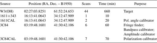
The observed sources. Sources ending in -CAL' are wide-band continuum observations.
2.1 Very long baseline interferometry data reduction
Dual polarization spectral line reduction – also called spectral-line polarimetry – raises many problems. These are covered in detail in Kemball, Diamond & Cotton (1995), and in the books by Zensus, Diamond & Napier (1995) and Taylor, Carilli & Perley (1999). The procedure is summarized here.
The data were loaded into aips, applying all the standard digital and scaling corrections relevant to VLBA data. Then the data were examined in their rawest form to flag any obviously bad data. The calibration file produced on-line by the VLBA observation was combined with less frequently measured gain versus elevation data as determined from single-dish pointing observations.
Amplitude calibration of the data was performed in two ways: corrections for the continuum calibrators were derived from the system temperatures and gain curves provided by the VLBA operations team; gain factors for the line source were derived using the ‘template fitting’ method embodied in the aips task acfit. This provides flux densities accurate to a few per cent. The amplitudes were also corrected for the sampler biases that result from the differences in voltage threshold levels of the digital samplers at the various antennas; corrections were derived from the total power spectra.
The phases were then calibrated. First, parallactic angle data correction was performed because the VLBA antennas have alt-azimuth mountings. Then, the phase offsets between the different IF bands were determined. This was accomplished by determining the IF-dependent group delays and phases for a small period of data on the calibrator 3C84. These corrections were applied to all data thereby removing all electronic offsets between observing bands. At this point, it was discovered that the Pie Town antenna was not giving acceptable fringes on its baselines, so the antenna was dropped from the data.
The task cpass was used to determine the complex bandpass corrections, again using 3C84 as a calibrator source. The residual Doppler motions of the Earth around the Sun and the peculiar motions of the Sun, relative to a circular orbit around the centre of the Galaxy were removed.
Because the observation was intended to detect linear polarization angles, the extra stage of polarization calibration was needed. For this, the wide-band data on the calibrator sources were used. The calibration procedure determined and corrected for three different factors, as follows.
The time delay between the lhc and rhc signal paths.
The phase offset between the two polarizations. If uncorrected this will result in a constant rotation angle being applied to the linear polarization vectors. Comparison with a calibrator source of known position angle is required. For this purpose, the source 1611+343 was mapped. This source remains a point source, even at VLBA resolution. The polarization position angle was measured to be −9°, but was known to be 32° from recent Very Large Array (VLA) observations.
Correction of feed impurities (‘D-terms’; see Kemball et al. 1995). The D-terms were corrected using data from the calibrator source 3C84.
2.2 Image creation
The next stage of calibration was to select a phase-reference channel on W3(OH). A strong channel, with simple structure, at 1665 MHz was selected. Its visibilities were fringe-fitted to determine the residual phase and phase rates caused by atmospheric fluctuations and any errors in the geometric model used in the correlator. Self-calibration was then performed to remove the effects of source structure from the channel visibilities. The corrections derived were then applied to all spectral channels and all bands thus anchoring all images to the centroid of the structure of the reference channel. imagr was then run for each Stokes parameter for each frequency to produce the final cleaned and calibrated map cubes. The first four channels and the last five channels of each band were flagged; they contain high noise because of bandpass limitations.
In order to cover the whole W3(OH) region, and to find any outlying masers, a 4 × 4 arcsec2 field of view was needed. In 1997, the maximum image size that was computationally feasible was 2048 × 2048 pixels, which would imply a cell size of 2 mas. For good sampling this would itself imply a beam size of ∼8 mas. Hence, the field of view desired could not be achieved without compromising image quality at the maximum resolution. To achieve the field of view with good image quality required a factor of 2 decrease in resolution by using a u, v‘taper’ in imagr to weight down the u, v, data outside a circle of radius 20 000 kilolambda (3600 km). A declination shift south, of 1 arcsec, was also added because the phase-reference feature was in the north of the map.
The observation was not externally phase-referenced, and so the absolute position of the phase centre cannot be determined to accuracy greater than 0.1 arcsec. However, observations of W3(OH) with the Multi-Element Radio Linked Interferometer Network (MERLIN) array at 1720 MHz in 1993 December that were phase-referenced were available (Gray et al. 2001), and were used to determine the absolute position of the phase centre, giving a position of  (J2000). The MERLIN absolute position has an intrinsic error of 10 mas, but additional uncertainties arise from the possible motion of the 1720 maser with respect to the 1665-MHz reference maser in the three years between the observations. There is little doubt that the MERLIN reference maser has been correctly identified, but the absolute motion of the maser is unknown. The maximum likely speed of any maser is ∼20 km s −1, or 2 mas yr −1. Over 3 yr, this is a maximum likely motion of 6 mas. The accuracy with which the positions of features at different OH transition frequencies can be determined is limited by the errors in the determination of the group delay. Measurements of this quantity on the calibrator sources suggest a maximum error of 20 ns. Combined with other possible sources of error, this introduces a positional uncertainty of no more than 100 microarcsec.
2.3 Measuring the maser emission
Because maser sizes are usually at or around the resolution limit, fitting two-dimensional Gaussians to the patches of maser emission typically collects the flux very well and gives very accurate values for peak flux density, total integrated flux and position. For fitting the Gaussians, the aips task sad was used. Although parameters in sad account for the widely varying flux densities of the peaks, it does sometimes fail and, in particular, it leads to very strong peaks with slight deviations from Gaussian form being broken up into multiple smaller peaks that may not represent reality. Where Gaussian fitting was consistently failing on intense and slightly extended masers, parameters were changed in an attempt to allow a more approximate fit to one Gaussian. For solid guarantee of a real detection, the detection threshold for masers is usually considered to be 5σ. The typical measured rms in the maps was about 15 mJy, so a value of 75 mJy was appropriate for the 5σ value.
The development aips task mfquv (written by D. Boboltz) was used after sad to search through the Stokes Q, U and V cubes using the Gaussian data already determined from the Stokes I cube. mfquv reads the position of every Gaussian fit in Stokes I and then measures the single pixel flux density at the corresponding position in the other three Stokes cubes. This has advantages over fitting Gaussians to every Stokes cube in turn (as well as being much faster), because it allows measurements of flux density to be made right down to the noise level. Only a small number of masers would have linear polarization fluxes above the 75-mJy threshold but, having already fitted the masers in Stokes I linear polarization, fluxes in Q and U can still be measured even if they are below the threshold for Gaussian fitting. These measurements will, of course, be subject to larger errors at lower signal-to-noise levels. mfquv is also useful because it avoids having to fit both positive and negative flux Gaussians in the same map (which is not currently possible with sad). It should be noted that, where masers are closely overlapping, mfquv might return incorrect values for fluxes. This is because sad performs Gaussian fitting on the Stokes I data, taking into account flux increases caused by overlap of adjacent masers, but mfquv just reports pixel-value fluxes for Q, U and V at positions provided by sad, without calculating any fits itself. In this way, polarized flux (from Stokes Q, U or V) may be effectively counted twice. This may lead to a slight overestimate of the polarized contributions in such cases – possibly taking the total polarized flux above the Stokes I flux (i.e. >100 per cent polarization). Fortunately masers are rarely this close to each other. Clearly, because many errors are related to the signal-to-noise ratio, for intense masers the estimated errors are much smaller than for weaker masers. Typical uncertainties for masers of different intensities are shown in Table 2.
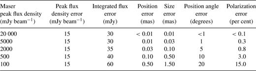
Typical errors as output by SAD for masers of an example range of peak flux densities. These numbers assume that the noise in the maps is ∼15 mJy beam-1, as it is in most channels.
However, by far the largest cause of uncertainties is circumstances where masers are closely overlapping. The Gaussian fitting of the masers is then at least partly dependent on the parameters chosen for the fitting criteria, and may produce significantly different results with different parameters. In such cases, the error on fluxes may be as high as 10 per cent, and the error on positions may be nearly the size of the beam (for resolved emission), ∼8 mas. In general, the accuracy of fit parameters for masers in complex areas of emission and well-resolved extended masers should be treated with some caution, while isolated and unresolved masers have errors that approach the theoretical minima.
Adopting the typical standard in this area, a candidate maser (called a ‘feature’ hereafter) would require detected emission in three consecutive channels, each within a certain spatial separation (‘tolerance’) of its neighbours. In order to collect the Gaussian fits output by sad, a fortran program called happy was developed. happy takes the strongest emission Gaussian fit in the given channel map and looks in the next channel map above for the nearest Gaussian spatially within the tolerance. Below tolerances of 4 mas, the maser features rapidly broke up and were dropped because they failed to achieve three consecutive channels. In the end, the tolerance was set at 4 mas, but the output of features from a tolerance of 6 mas was examined manually as well, to identify any masers in areas of complex emission that were being lost at 4 mas but that ought to be kept. Peak Stokes I flux densities were used throughout when generating the full I, Q, U, V data set via the task mfquv.
2.4 Line shape fitting
Fits to a line shape may be optimized to one of two possible quantities: the total integrated flux of the Gaussian fit (in Jy) and the peak brightness (in Jy beam −1). The latter is better for investigating the properties of individual maser line shapes because it reflects the intensity at the centre of the maser, while the total integrated flux reflects the intensity over the whole of the maser – and so is easily influenced where masers are overlapping. Indeed, the total integrated flux is more useful where it is suspected that a maser feature may in fact be an unresolved double feature, because this often shows up in the line shape as a ‘shoulder’ on the main peak, whereas the peak flux density line shape is less influenced by this unless the masers are extremely close.
It is clear that sad and happy, either on their own or together, do not form a ‘black box’, and so the output of both was checked at every stage to make sure that the generated features had a strong foundation in the maps.
Next, dynamic-range-induced amplitude errors were removed manually from the feature list generated by happy. These amplitude errors affected channels with strong maser peaks, in particular 1665-MHz channels 59–63. In the images, the amplitude noise often follows symmetrical patterns, especially ripples that centre on the intense maser causing the dynamic range problems, and such patterns were visible in the early plots of the feature positions. The majority of such spots were eventually eliminated.
2.5 Zeeman pairs
It has long been known that the similarity of right circular polarization (RCP) and left circular polarization (LCP) emission from maser areas, as detected by single-dish observations, is caused by the Zeeman effect splitting and shifting the two spectra apart. The identification of Zeeman pairs provides much more useful information than individual Zeeman components because, without pairs, no conclusive values can be placed upon the true velocity of the masers. This is because the magnetic field strength is both unknown and variable across the source.
Having cleaned the data of systematic effects, those features which had been rejected earlier by happy for having just two adjacent channels were reincluded into the data for the purposes of seeing if any were the weaker component of a pair. Their inclusion here was justified, because in order to be a Zeeman component the feature would have to lie within a very small area, within a certain range of velocity (determined by the knowledge that the magnetic field ranges between ∼1 and ∼20 mG) and be of opposite polarization. Naturally, a tolerance value had to be adopted, within which Zeeman components could be considered associated. It was decided that there would be two classes of Zeeman components: class a would be the highest confidence associations where all components were within 6 mas of each other; class b would be lower confidence associations where all components were between 6 and 12 mas of each other. In only two instances were candidates for π components or Zeeman triplets found, all the rest were σ± Zeeman pairs. This is not surprising because only one convincing example of a complete Zeeman triplet has been discovered (Hutawarakorn, Cohen & Brebner 2002). All Zeeman pairs where one component had only two channels were declared to be quality b, regardless of their separation.
2.6 Demagnetization and magnetic field strengths
Having identified Zeeman pairs, the process of extracting the extra information contained in them can begin. The first of these processes was ‘demagnetization’. This allows the determination of the true velocity of the maser from the velocity of its two components. In order to do this, the velocity of each component needs to be determined. Where a maser had been successfully fitted with a line shape, the value of the Gaussian mean was used, and the standard error of the Gaussian was used as the error in the velocity. Where a fit had not succeeded, because either there were less than four points in the line shape or the line shape was not sufficiently Gaussian, then the velocity of the peak channel was used. The value of the velocity in a channel is the mid-point of that channel, and therefore the error was estimated at 0.5 channel widths. Demagnetization is then simply the averaging of the two component velocities. The errors on Gaussian-fitted spectra were also typically about 0.5 channels. Because the velocity of a channel is taken at its mid-point, the maximum uncertainty can be half a channel each way. Very weak features could, however, have formal uncertainties in velocity of greater than 0.5 channels; where this was so, the error was set to 0.5 channels, because it would have also been possible to just use the velocity of the peak channel and obtain a lower uncertainty.
The magnetic field strength in the maser is found by a similar method to the demagnetized velocity. When the Zeeman components are more widely split than the FWHM of each component, the magnetic field strength is related to the separation of the peaks. Using the component peaks and errors as in the demagnetized velocity calculation, the magnetic field strength, along with an error, was calculated for every Zeeman pair. Because the magnetic field is proportional to the Zeeman splitting, the fractional error in the field is equal to the fractional error in the velocity separation of the peaks.
2.7 Proper motion
The absolute proper motion of the masers cannot be determined because of the relatively large error in the absolute position determination of this and previous observations compared to the presumed size of the proper motion. However, the proper motion of the masers with respect to a reference maser can be calculated with great precision if the reference maser can be identified in observations at two or more epochs. Identification of such a maser in the data of Bloemhof et al. (1992) was easy; that work had successfully performed a proper motion measurement that would also allow a good comparison. Their method was used to calculate the proper motions, with the additional conversion of B1950 coordinates to J2000 coordinates using the Rutherford Appleton Laboratory's coco v2.2-3 software utility in high-resolution mode. The resulting proper motions were in the range ∼3–13 mas over the 19 yr between the observations.
2.8 Two-point correlation
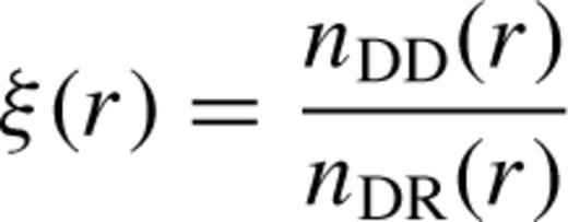
The correlation was performed with only one maser from each Zeeman pair. Because both masers in a Zeeman pair are effectively the same maser, only the position of the stronger maser was entered into the correlation. If both masers had been entered from every pair, then the correlation would have shown a huge spike below 12-mas scalelengths where the correlation between the components of each pair dominated.
3 ANALYSIS OF W(OH): 1665 MHz
Fig. 1 shows the Stokes I spectrum of the maser fluxes calculated from the channel maps. The 1665-MHz maser spot map is shown in Fig. 2. As is immediately apparent, the 1665-MHz map is exceedingly complex, featuring 211 detected masers. There is no immediately obvious pattern to the distribution (other than that the masers cover only the western half of the H ii region), although there is an indication of clustering. The most intense masers (i.e. >10 Jy) appear in the north or in the south, with just one intense maser in the centre.
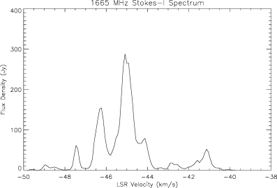
The Stokes I spectrum of the maser fluxes calculated from the channel maps.
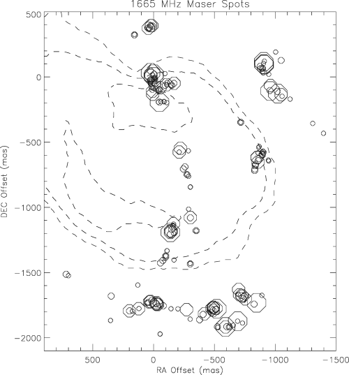
The 1665-MHz maser spot map. Contours are the 0.5, 7.1 and 16.6 mJy beam −1 levels of a VLA 2-cm continuum map (Masheder et al. (1994) and references therein). The spots are divided into four classes, represented by symbols of different sizes. In order of increasing symbol size, and maser flux, these classes are: (i) <0.4 Jy; (ii) 0.4–2.0 Jy; (iii) 2.0–10.0 Jy; (iv) >10 Jy.
3.1 Comparison with previous work at 1665 MHz
Comparing the spectra of 1978 (Garcia-Barretto et al. 1988), 1986 (Bloemhof et al. 1992) and 1996 (this work), it is seen that the 1665-MHz emission has remained fairly similar in form, with the notable exception that the very bright RCP emission at −45 km s −1 appears to have faded in flux. The distribution of masers from 1978 and 1986 matches excellently with that in Fig. 2, indicating that the 1665-MHz maser groups are relatively stable features.
Caution needs to be exercised when comparing the flux densities because of the possible effects of different fitting procedures and different sized beams, but it was immediately apparent that the masers are indeed noticeably variable over a decade time-scale. The matching of component position angle at different epochs was not attempted, because this is very much dependent on how complex areas of maser emission have been broken down during fitting. Only five of the 45 masers listed in Bloemhof et al. (1992) could not be found in the current data. The brightest of these in 1986 (15 Jy beam −1) is probably now obscured by the much brighter masers in the complex north-western group. The remaining missing masers have relatively low fluxes and could have all faded since 1986. Bloemhof et al. (1992) detected a trend towards lower flux densities – peaks in 1986 were on average 80 per cent of the peaks in 1978. They suggested that this could be explained by a flux density miscalibration of 20 per cent at either epoch. This trend continues, however, into the current data – flux densities in 1996 were on average 75 per cent of those detected in 1986, and 60 per cent of those in 1978. It is unlikely that this is an accidental result of miscalibrations, but instead a real secular trend reflecting the limited life of the masers. However, we cannot rule out maser brightness fluctuations on time-scales much shorter than the typical interval between the observing epochs. It appears that maser groups are stable features, whilst individual masers within a group may come and go over a time-scale of decades. A similar effect was noted in Desmurs et al. (1998)– observing at the 6-GHz excited state – that, in comparison with Moran et al. (1978), the general distribution of maser groups had been preserved but there were many changes in the major components. This would suggest the scenario where ‘maser-friendly’ conditions persist on the large scale in certain locations for many decades, but individual masers have a lesser lifespan of just a few decades. One maser had brightened by 47 Jy beam −1 in two decades since the Garcia-Barretto et al. data were taken.
3.2 Maser morphology
Some patterns in the morphology of the masers are immediately apparent. Most notable was the extended nature of the masers in the centre-west of the map at offset coordinates −0.85 arcsec RA, −0.65 arcsec Dec.; these masers have a relatively long average major axis of about 12 mas, and relatively low brightness temperatures. They are generally elongated in the north-west to south direction; of the masers brighter than 0.5 Jy, nine out of 11 have position angles in the range from 155° to 179°. Images of these masers appear in Fig. 3. Also apparent is that in the extreme north and south of the map, the masers tend to be elongated east–west; in the south, this east–west orientation follows tentative lines or arcs of masers which may indicate shock fronts (see Paper II).
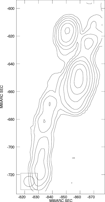
Masers displaying elongated morphologies. A Stokes I image of the maser group at offset coordinates −0.85 arcsec in RA, −0.65 arcsec in Dec. (maser group d). Nine of the 11 features, with fluxes >0.5 Jy, identified in this group have position angles in the range of 155°–179°.
The masers near the reference feature are typically small and often unresolved; these masers have an average deconvolved major axis of 4.5 mas, and have relatively high brightness temperatures. The complexity of emission at 1665 MHz makes Gaussian fitting very difficult in some areas because the masers are blended. Fitting was extremely difficult in the crowded southern areas of emission, and in the far north-east. In the north-west are some very intense and large masers where two of the masers merge completely, resulting in a maser fragment, and a complex line shape for this feature because it has effectively ‘consumed’ another maser.
3.3 Maser line shapes
Examination of the 1665-MHz line shapes is complicated by the number of masers in close proximity to each other, which can often lead to distorted line shapes where any outlying flux from one maser adds to the peak of its neighbour.
Of particular interest are the maser line shapes that are not approximated by a Gaussian line shape. Theoretical modelling of maser line shapes has been performed by several authors (e.g. Bettwieser & Kegel 1974; Goldreich & Kwan 1974; Bettwieser 1976; Nedoluha & Watson 1988; Elitzur 1990; Nedoluha & Watson 1991; Wu 1992; Wu & Elitzur 1992; Field, Gray & de St Paer 1994). Work by Nedoluha & Watson (1990) and Field et al. (1994) has predicted that saturating masers may evolve into complex or multipeaked line shapes.
Of the 211 masers detected at 1665 MHz, 87 failed fitting with a Gaussian line shape. A minimum of four points was required in the line shape for an attempt to be successful. Table 3 indicates the numbers and reasons for failure of line shape fitting. The spots allocated as ‘probable unresolved double’ have the attribute of being morphologically elongated and, typically, the maser centre moves noticeably through the frequency channels, indicating that a second maser probably sits only slightly offset in both position and velocity.
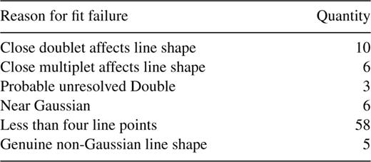
The -MHz masers that failed to be fit with Gaussian line shapes.
Of the five masers with genuine non-Gaussian line shapes, two are weak peaks in noisy areas, and are likely not reliable. The other three are shown in Fig. 4. Feature 97 has an excess of emission in one line wing. This type of behaviour could result from the growth of emission in the line wing where the optical depth is greater. All three features shown in Fig. 4 are probably saturated; brightness temperatures for features 97, 64 and 359 are 2.4 × 10¹¹, 9.8 × 10¹¹ and 4.5 × 10¹⁰ K, respectively. If these features are amplifying the continuum radiation from the optically thick H ii region, a reasonable background temperature is 104 K. The smallest amplification factor of the three, for feature 359, would then be 4.5 × 10⁶, and we expect masers to saturate at smaller amplification factors than 106 (Gray & Field 1995). Normally, the line rebroadening following saturation would be symmetrical, and both wings would grow, but if conditions are slightly less favourable for masing in different parts of the maser, then rebroadening may be suppressed in one wing. Feature 359 appears to be a true double peaked maser. Such a line shape is what would be expected from the phenomenon of ‘hole burning’ (Field et al. 1994), which can occur in a maser under ‘negligible velocity redistribution’ (NVR) conditions such that the line centre may go into anti-inversion. The fact that just one single maser out of 211 exhibits this type of line shape suggests that NVR conditions are very much the exception in 1665-MHz star-forming region masers.
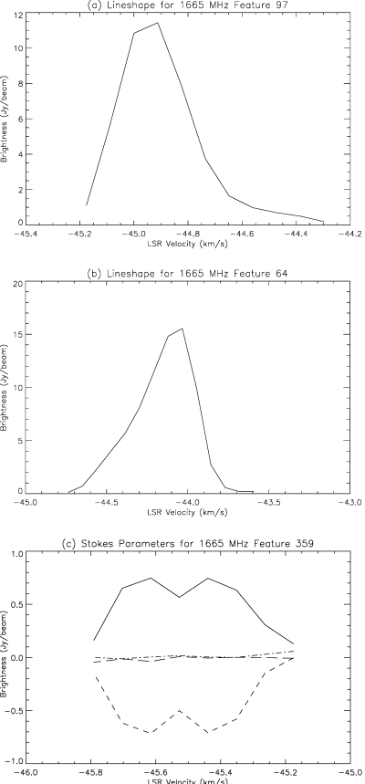
Distinctive non-Gaussian maser line shapes. The Stokes parameters are shown for feature 359 (Fig. 4c) to emphasize that it is not an overlapping LCP and RCP maser. The spectra for the Stokes parameters in this, and all subsequent diagrams, are represented by: solid line, I; long-dashed line, Q; chained line, U; short-dashed line, V.
This leaves the interesting feature 64, also shown in Fig. 4. This is a very dynamic maser, which has been rapidly declining in intensity in the last two decades. It is by far the most intense maser with a non-Gaussian line shape – with Tb of 1012 K it is definitely of saturated intensity, and the deviation of its line shape from Gaussian is the largest of any maser. It is also unusual in that it has changed velocity in the last decade; typically, masers may move spatially, brighten or fade, but they remain constant in velocity. Indeed, this is usually the best way to identify masers between epochs; the average change in frequency of the peak of masers identified in the data of Bloemhof et al. was 0.08 km s −1, which is less than one spectral channel. The change in velocity, position and intensity of this maser was first noted by Norris & Booth (1981), who measured the changes relative to feature 271. In the 1978 data, it had a peak velocity of −43.78 km s −1 (Garcia-Barretto et al. 1988). In 1996, the velocity of its peak was −44.03 km s −1, a change of −0.25 km s −1 from the 1978 value. Only two other masers have a velocity change of this magnitude, both in the far north-west cluster, which may be partly due to the difficulty of resolving the complex emission there. Nevertheless, the trends detected above are in agreement with those of Norris & Booth (1981). Over a period of 19 yr, this velocity change represents an acceleration towards us (or a deceleration away from us) of 13 m s −1 yr −1. This velocity shift could also be caused by a decrease in the maser cloud magnetic field of 0.8 mG (about 10 per cent for this region, see Section 3.5), or 0.04 mG yr −1. However, given that magnetic fields in star-forming regions are coupled to matter (e.g. Shu, Adams & Lizano 1987) this would require the maser cloud to be expanding. Given the unusual nature of this maser's line shape and its acceleration, it may be reasonable to assume that the phenomena are connected; possibly this masing cloud is experiencing a collision.
3.4 Polarization
Garcia-Barretto et al. (1988) studied W3(OH) in full polarization. They found the vast majority of masers to be ∼100 per cent circularly polarized, except in the area to the far north-west. Here, many of the masers showed relatively high linear polarizations and also some unpolarized emission. Outside this area, just six of 71 masers were significantly less than 100 per cent circularly polarized. They found 41 (58 per cent) LCP and 30 RCP masers.
Of the 211 masers detected in 1665 MHz in the present data, 122 (58 per cent) are left elliptically polarized and 89 right elliptically polarized. 154 (74 per cent) have greater than 90 per cent circular polarization. Of the masers with peak flux density over 1 Jy beam −1 the last statistic rises to 68 of 80 (85 per cent). No masers exhibit more than 50 per cent linear polarization. In terms of linear flux density, only seven masers have brightnesses higher than 0.35 Jy beam −1; these are shown in Table 4. As explained in Section 2.3, the polarization figures become less reliable as the flux decreases, such that the error is potentially ∼10 per cent by 0.2 Jy beam −1.
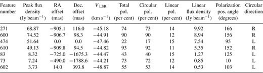
-MHz masers with high linear polarization. Information shown is for the peak channel in the maser feature.
The top four masers in Table 4 are also the top four in total flux density, one of which is the reference feature. Values for feature 602 should be considered with caution because it merges with another feature; this will have an effect on the line shape and polarization values. Feature 600 also has a merger with another feature. The Stokes line shapes of the four unhindered features are shown in Fig. 5. The top two and bottom two in Table 4 have Zeeman partners, all of which are much the fainter of the pair.
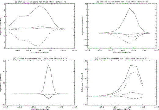
Stokes spectra of simple 1665-MHz masers with high linear flux densities. To relate line styles to the Stokes parameters, see the caption to Fig. 4.
Feature 73 (Fig. 5a) is probably an unresolved double, which leads to the shoulder on the blue end of its spectrum. Features 83 and 474 (Figs 5b and c, respectively) are striking because most of their emission is unpolarized. Only 16 of the 211 masers are less than 50 per cent polarized, all in the far north or south of the map. There are two that are 10 per cent or less circularly polarized, and both of these are in the interesting region to the extreme north-east of the map. The masers of this region typically have low total polarizations and moderately high linear polarizations. Only four (weak) masers have more linear than circular polarization. It is still assumed that these are σ components, although they are amongst the most likely candidates for any π components in the map.
In two places, at offsets of ∼(24, 394) mas and ∼(−725, −1679) mas, three masers were found within 12 mas of each other (the criterion for possible Zeeman triplets). The two cases are shown as Stokes plots in Fig. 6. In case (a) the central peak is not mid-way between the other two, so a Zeeman triplet is unlikely; this could simply be a Zeeman pair and a Zeeman singlet coincident. For the purposes of magnetic field measurement, features 51 and 376 were taken to be the Zeeman pair. Notice, however, that in feature 83 the linear polarization (Stokes Q and U) peaks nearer the centre of the Zeeman pair than the circular and unpolarized emission. It is very hard to see how feature 83 could be a π component because it has a significant intensity in Stokes V. In case (b) the situation is more unusual. The RCP component (feature 629) has only a tiny fraction of circular polarization (0.5 per cent), and is perhaps the best candidate for a π component in the data, purely on this criterion. If interpreted as a π component, it gives a magnetic field measurement well out of the ordinary for this maser group, because it cannot form a triplet with both the features 505 and 603; a triplet would require an additional feature as a σ-type companion to either 505 or 603, displaced some 3 km s −1 to the red of feature 629 itself. Therefore, feature 629 is still interpreted as a RCP Zeeman component, paired with feature 505. If both the LCP emission peaks are from the same individual maser, then the LCP component has been split, possibly by a large velocity gradient within the maser. The polarization angles of the masers in both cases do not add any weight to their interpretation as Zeeman triplets. Overall, we found no convincing candidates for π components.
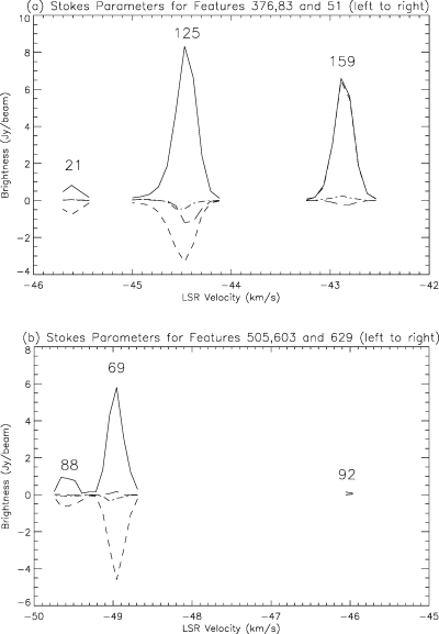
The two candidate 1665-MHz maser Zeeman triplets. Numbers within the figures are polarization angles in degrees.
The third case with slightly ambiguous Zeeman interpretation is that of the southernmost maser emission detected at (−53, −1972). The brighter of the two masers is largely unpolarized, with less circular polarization than linear, while the weaker is a fairly typical RCP maser. The separation between the peaks gives a sensible magnetic field value if interpreted as a π component and one σ component. In addition, the angular difference of the polarization angles is 98°; close to the 90° that would be expected.
Fig. 7 shows the variation of polarization with RA and Dec. Only masers with flux density greater than 750 mJy beam −1 are included to remove those with large uncertainties. A possible trend emerges in Dec. (Figs 7a, c and d): the curves are least-squares quadratic fits, shown simply to illustrate the nature of the trend. There is no clear trend in RA (Fig. 7b). In general, total polarization and circular polarization are closely tied. This means that, moving to the north and south, the amount of unpolarized and linear emission in the masers increases. An explanation for this picture of changing polarizations moving away from the centre of the region is that the angle of the magnetic field with respect to the line of sight is increasing as we move away from the centre of the map. Because the molecular gas surrounds the approximately spherical UCH ii region, a simple model where magnetic field lines in the gas point generally towards the central star would satisfy this proposition, whether the gas was in a shell/envelope or a torus.
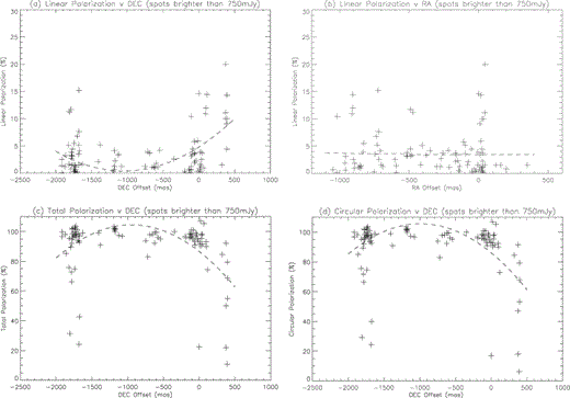
The variation of linear polarization with RA and Dec., and the variation of circular and total polarization with Dec. Curves are least-squares fit quadratics.
The projection of the angle of the field on to the sky could be deduced from the angle of linear polarization of the masers that contain a reliable linear percentage, but there are certainly no obvious trends in the data. On closer inspection, it can be seen that on small scales the masers are often aligned with their neighbours. This is most clear in regions that have the highest fraction of linear polarization. Also, of the 88 masers with linear intensities greater than 30 mJy beam −1, 30 have polarization angles of 0 ≤θ < 90, while 58 have polarization angles of 90 ≤θ < 180. The probability of this, or a greater, imbalance occurring by chance is only 0.0014 on the basis of a normal distribution, which indicates that the large-scale cloud field probably has a north-west to south-east alignment. The error in polarization position angle measurements depends on spot intensity, but for those spots considered here, it is typically less than 2 °.
The symmetry of the variation in polarization percentages with Dec. most likely reflects a degree of north–south symmetry in the structure of W3(OH). The OH masers have previously been predicted to lie in a north–south torus about the UCH ii region (Harvey et al. 1974), a shell around the UCH ii region, or in matter in front of the UCH ii region, Reid et al. (1980); (Norris & Booth 1981). In any case, the first two of these cases would automatically exhibit north–south symmetry.
Current maser theories do not predict the large amount of unpolarized emission coming from masers that are presumed to lie in gas where the magnetic field is at a high angle to the line of sight. The probable cause is Faraday depolarization in the presence of high electron densities, or long maser path-lengths giving higher electron column densities. Longer path-lengths might be expected at the edges of a spherically symmetric region of gas. Nedoluha & Watson (1990) show that the overlap (or blending) of Zeeman components could cause the linear polarization to cancel, giving unpolarized emission, but this does not explain how unpolarized emission could be present in a separated Zeeman pair where the components are clearly not overlapping.
3.5 Magnetic field structure
58 Zeeman pairs were found, which are listed in Table 5. This means that 55 per cent of the masers are members of a Zeeman pair. The distribution of Zeeman pairs is illustrated in Fig. 8, which shows that the Zeeman pairs appear to be a fairly random selection of masers over the map, with all maser groups well represented. When analysing the properties of the masers, it is convenient to separate the W3(OH) map into groups of masers which appear clustered, shown in Fig. 8. For the symbols used to identify the groups, see the caption to Fig. 8. At this stage the divisions are based solely on apparent spatial association, but it will be seen that the divisions probably represent underlying maser associations, with similar physical conditions. Our classification of maser groups is therefore different from, and simpler than, that found in Reid et al. (1980), which was based on selection of bright emission regions for observation at high resolution, an observational necessity at that time. We note that the subregions used by Garcia-Barretto et al. (1988) and Bloemhof et al. (1992) are based on those defined by Reid et al. (1980). A total of 23 features were found outside the mapping regions defined in these earlier papers.
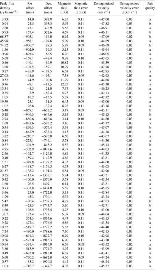
-MHz Zeeman pairs. Information for peak flux, RA and Dec. are from the peak channel in the brighter of the two Zeeman components.
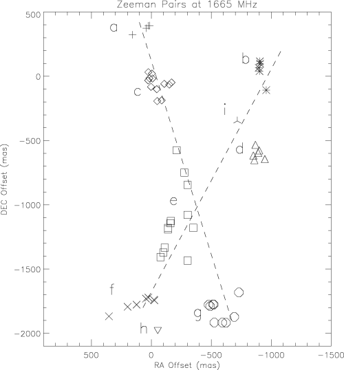
1665-MHz Zeeman pairs in W3(OH), with symbols denoting maser groups (see text). The symbols are allocated to the maser groups as follows: plus sign for a; asterisk for b; diamond for c; up-pointing triangle for d; square for e; cross for f; octagon for g; down-pointing triangle for h; three-point symbol for i. The dotted lines are at +18° and −30° to north.
The median ratio of the fluxes of the Zeeman pairs is 4.4:1. The mean is heavily distorted by the Zeeman pairs containing the two brightest masers, which have very weak Zeeman partners and so have flux ratios in the hundreds. The mean including these two ‘outliers’ is 17.8:1; after dropping them, it is 6.9:1.
The variation of magnetic field strengths with RA and Dec. is shown in Fig. 9. This shows clearly the exceptional nature of maser groups c and d. The peculiar magnetic field characteristics of these two groups has already been noted in Garcia-Barreto et al. (1988). Group c is the only group where there are large variations in magnetic field, and the field within the group is generally strong. Group d is exceptional for essentially the opposite reasons: the remarkable constancy and general weakness of the magnetic fields. The field characteristics in the maser groups are shown in Table 6.
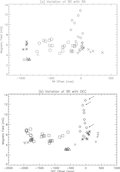


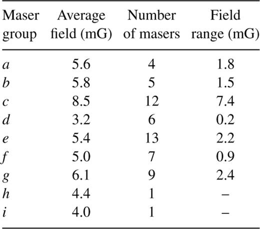
Magnetic field properties of the different maser groups. Overall average is .9 mG.

The tendency of most maser groups to have magnetic fields in the region of 4–7 mG is in good agreement with previous magnetic field measurements at 18 cm in W3(OH) (e.g. Moran et al. 1978; Reid et al. 1980; Garcia-Barretto et al. 1988; Bloemhof et al. 1992), and also with measurements at the 6-GHz (5-cm) excited state in other star-forming regions (e.g. Baudry et al. 1997; Desmurs & Baudry 1998). However, the seven field measurements weaker than 2.5 mG that Bloemhof et al. recorded were not reproduced. Four of these have quality codes that bring their identification as Zeeman pairs in Bloemhof et al. into some doubt; for example, one pair listed as quality D by Bloemhof et al. has a component separation of some 40 beam widths. For the remainder, Bloemhof et al. suggest that there is considerable uncertainty in the Zeeman interpretation; in the light of the new results it is probable that these were not in fact Zeeman pairs. Notably, the two largest field values recorded by Bloemhof et al. (8.2 and 9.1 mG) are located in region c. The relatively high magnetic field strengths in group c are in agreement with excited state OH masers measured at 6 GHz (Moran et al. 1978, Desmurs et al. 1998) and at 13 GHz in Baudry & Diamond (1998). In Desmurs et al. their region 1 has the highest magnetic field strengths (average 7.6 mG at 6035 MHz, 9.7 mG at 6031 MHz) and corresponds in position to maser group c in this work. In Baudry and Diamond, masers at 13 GHz are found only in the small area corresponding to maser group c, and field strengths vary between 5.6 and 11.3 mG with an average of 9.6 mG, in excellent agreement with a range of 5.4–12.8 mG for maser group c.
It is worth noting also that the average field for group d (3.2 mG) is close to that detected by Güsten, Fiebig & Uchida (1994) in thermally excited non-masing gas in absorption against the radio continuum. They measured a line-of-sight component field of +3.1(±0.4) mG. However, from the polarization data in the previous section, the magnetic field direction is most likely near to the line of sight across much of the face of the UCH ii region, and so their figure may be approaching the total field strength of the dense non-masing gas in front of the UCH ii region. This would mean that group d has conditions closest to the non-masing gas around the UCH ii region. In this case, group d may be just forming from the gas, or dissipating into the gas. In either case, the conditions in the gas in group d are probably significantly different to those in group c, which shows the greatest difference in conditions to that in the ambient gas. The relatively low magnetic field measured in i suggests that it may be the closest in conditions to group d. Zeeman pair h should be considered tentatively; its Zeeman nature is open to interpretation, as discussed in the previous section.
The strength of the magnetic field in maser group c has implications for the phenomenon of Zeeman component overlap as suggested by Nedoluha & Watson (1990), which sought to explain the suppression of one Zeeman component. The Zeeman splitting of 12 mG at 1665 MHz is ∼7 km s −1. According to their theory of component overlap, this means that the velocity shift across the maser must be of this magnitude or larger, which is unreasonable because this is approaching the velocity extent of the entire source. An individual maser is very much smaller than the whole source, and turbulent eddys of a size similar to a maser should therefore have characteristic velocities considerably smaller than 10 km s −1, characteristic of the W3(OH) maser region. Nedoluha and Watson themselves suggest that the 3–4 km s −1 splitting previously detected must be at the high end of what is plausible. It could be argued that we will tend to see Zeeman pairs in regions of high magnetic field, and single components in areas with low fields where overlap is plausible. With this in mind, we might expect to see fairly equal fluxes (low Zeeman ratio) in the components of Zeeman pairs in a high-strength field because it is unlikely that sufficiently large velocity shifts will be found to cause enough overlap to diminish one component. Fig. 10 shows no such correlation.
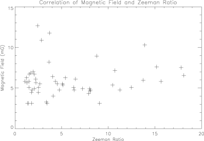
Magnetic field strength of Zeeman pairs versus their ‘Zeeman ratio’ (the ratio of their peak flux densities).

3.6 Velocity distribution
Every Zeeman pair can be reduced to a single maser at the true gas velocity in the local standard of rest (LSR) frame of the experiment. Fig. 11 shows the variation of these demagnetized velocities with Dec. (Fig. 11a) and RA (Fig. 11b). The distribution with Dec. shows a clear trend, rarely mentioned in W3(OH) literature (the trend is apparent in much previously published W3(OH) data but was not commented on since Harvey et al. 1974, although Guilloteau, Stier & Downes 1983 hinted at it). The north of the cloud is moving towards us faster than the south. The UCH ii region is optically thick at the L band (e.g. Kawamura & Masson 1998), so the maser emission certainly comes from the near side of the region. The dotted line on the graph is a least-squares fit plotted excluding maser groups c and h. We argue that this fit is significant on the following basis. The formal error on each demagnetized velocity is very small, amounting to 0.03 km s −1 (see Table 5). We cannot obtain a significant fit using these errors because, with velocities of such precision, we would require a high-order polynomial fit to obtain a reasonable value of χ2. However, the line we are fitting is a velocity gradient, so attached to each point should be an estimate of the velocity deviation of a given maser from the expected value for its declination, rather than the formal measurement error. These velocity deviations are probably dominated by random turbulent motions, but would also contain a component due to the overall expansion detected by Bloemhof et al. (1992). As an estimate of these deviations, we have taken the standard deviation of the demagnetized velocities in each group; in the case of group i, which has only one point, we have kept the formal velocity error. The largest of these standard deviations, for group b, was 0.867 km s −1, and the smallest was 0.209 km s −1, in the case of group d. Using the group standard deviations as our uncertainties on each point, we obtained the following fit parameters: intercept, C =−46.111 ± 0.049 km s −1; gradient, M =−1.607 ± 0.095 km s −1 arcsec −1; χ2 = 46.50. This last quantity yields a quality factor of 0.33.
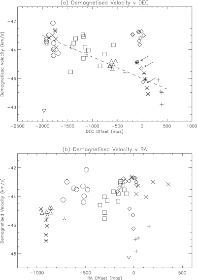
Variation in ‘demagnetized’ velocity with (a) Dec. and (b) RA in W3(OH). The arrowed points are indicated for comparison with Fig. 9. In velocity, the arrowed points appear possibly part of the main velocity trend, but in Fig. 9 it is clear that their field strengths are well above any others in the main trend; so they are definitely part of maser group c. For symbols identifying the various maser groups, see the caption to Fig. 8.

The special nature of group c was indicated earlier with respect to the high magnetic field strengths there, and now this is reinforced by the fact that group c does not share the same velocity characteristics as the rest of the masers. The main body of group c has a velocity dispersion in agreement with the 13-GHz masers which are a coincident group; whilst at 6 GHz the large full spread is also observed in the region corresponding to group c. The other groups of masers at 13 GHz have velocities in good agreement with the 1665-MHz maser groups at coincident locations suggesting that they share the bulk movement of the 1665-MHz maser groups; whilst the 6-GHz masers share the bulk movement of the group c masers. The velocity gradient is also clear in the 6-GHz methanol masers (Menten et al. 1992), which also had a clump of masers over group c sharing the full velocity spread; and also in the 12-GHz methanol masers (Menten et al. 1988; Moscadelli et al. 1999), which share a generally similar position and velocity spread to the 6-GHz masers. If the two northernmost masers in the 23-GHz methanol group (Menten et al. 1988) are assumed to be in the main body of group c, with which they are coincident, then the velocity gradient is also apparent in the arc of masers to the south of them. Recently, the masers in our group c (group 2 in Reid et al. 1980) have been fitted with some success by a complex, seven-parameter conical outflow model (Moscadelli et al. 2002). The extent of the model is about 200 mas in each axis, so it is not relevant to the overall structure shown in Figs 2 and 8.
The location of maser group c is between a ‘pinch’ in the continuum emission – which could be caused by a denser clump in the outlying gas that is resisting ionization – and the northern peak in the continuum. Baudry & Diamond (1998) suggest that this might be the location of the O-type star powering the H ii region. This means that the star would be located away from the geometric centre of the continuum emission. Although this asymmetry seems unlikely at first sight, several pieces of evidence suggest that the site of the star is behind maser group c. The presence of 13-GHz OH masers Baudry & Diamond (1998) suggests higher densities than typically required for 18-cm masers (Gray 2001). In addition, Moscadelli et al. (1999) show evidence for a velocity gradient in the methanol masers that would lie within group c, and the high brightness temperatures at 12.2 GHz, compared to 6.7 GHz (Menten et al. 1992), is also evidence of higher densities near maser group c (Sobolev et al. 2002). The exceptional nature of the group h Zeeman pair is also clear. Fig. 11(a) also shows that, with the exception of group c, turbulent motions within each maser group are spread across ∼2 km s −1.
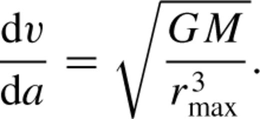
Circumstellar discs are believed to be common around stars (Hollenbach et al. 1994) and are known to contain large amounts of molecular gas (e.g. Beckwith & Sargent 1993). The idea of a rotating torus in W3(OH) has been suggested before (e.g. Harvey et al. 1974; Guilloteau, et al. 1983, who observed a velocity gradient in NH3 absorption). However, this has fallen from favour recently because of conclusive evidence of the expansion (or growth) of the UCH ii region (Kawamura & Masson 1998), which does not actually rule out a disc, and the conclusive evidence of divergent motion (Bloemhof et al. 1992), which does not rule out a disc either, although it does require that there must be some expanding motion in addition to ordered rotation. However, circumstellar discs have come back into favour following the work of Norris et al. (1998), who showed that half of a selection of methanol maser sources showed evidence for circumstellar discs. Many of these have OH and/or H2O masers present also, but have not been studied at high resolution, mainly because they lie in the southern hemisphere where the VLBA and European VLBI Network (EVN) have poor visibility. Only W3(OH) has been studied in detail in all the common molecular species, but Norris et al. (1998) allocated W3(OH) as ‘complex’ in their scheme because no simple linear structure could be found. However, in the light of the data above, concerning both the OH and the methanol masers in the area of maser group c, it is likely that W3(OH) is actually a combination of both ‘compact’ and ‘line’ in their scheme (the masers under group c being ‘compact’, the rest being ‘line’).
The mass of material around the UCH ii region has been estimated at 1 M⊙ by Guilloteau et al. (1983), and an upper limit of 3 M⊙ was set by Wink et al. (1994) using CO observations. Wilson et al. (1991) proposed a ‘cloudlet’ of 4 M⊙ containing the OH masers, which could itself be the disc. Hollenbach et al. (1994) concluded that discs of mass ∼0.3 M* exist around massive stars early in their history, which are then evaporated away by the star over about 105 yr. A north–south disc is attractive in W3(OH) because it can also explain why only the western half of the UCH ii region is populated with OH and methanol masers, excited-state OH absorption (Baudry & Menten 1995), formaldehyde (H2CO) and methyl formate (HCOOCH3) (all in Wyrowski et al. 1999). Interestingly, SO2 was detected only over the eastern half of W3(OH). A north–south disc would also explain the east–west elongation of the UCH ii region, because this would be the easiest path of escape for the ionized gas and outflows. No significant CO emission is detected over the UCH ii region (Wyrowski et al. 1997). An indication of a slight inclination of the disc in the plane of the sky can be seen in the arc-like nature of the easternmost OH masers at 1665 MHz, and in the methanol masers at 23 GHz. After noting that the variance of the distribution of maser positions is maximized along the Dec. axis, Bloemhof et al. (1992) suggested that the 10° angle of the arc represented the star moving into the plane of the sky at that angle for their cometry bow-shock model. Equally, this 10° angle could be the inclination of the disc to the line of sight, and this would explain how the western half of the UCH ii region is covered with molecular material. This slight inclination also has the effect of reducing the apparent rotation speed of the disc. A 10° inclination would reduce the measured velocity by just 1.5 per cent for simple Keplerian rotation, with the corresponding effect of increasing the mass estimates by 3 per cent.
At this point, the underlying systemic velocity of the star and UCH ii region becomes important; unfortunately, this is far from certain. Reid et al. (1980) took a value of −50 km s −1 from 22-GHz recombination lines (Hughes & Viner 1976) and, using this, deduced from the velocity centroid of the masers that they were in an infalling shell or accreting envelope. Using this value, all the maser groups would be infalling; those in the south falling the fastest, those in the north much more slowly. Infall on this scale is effectively ruled out by the divergent motion demonstrated in Bloemhof et al. (1992). However, the hydrogen lines are very broad (e.g. Sams, Moran & Reid 1996) and observations at higher frequencies showed that recombination lines at lower quantum numbers were redder. Berulis & Ershov (1983) showed that this effect could be caused by a rapidly expanding shell of ionized material moving at 18 km s −1, away from a central star at −46 km s −1. Welch & Marr (1987) observed that, at lower quantum numbers, the hydrogen recombination lines approached the maser centroid, and calculated a value of −45.6 km s −1 for the star. Keto Ho & Reid (1987) supported the infall model with evidence for both a rotating disc of NH3 and a collapsing shell of NH3, but poor resolution means that the emission cannot be definitely pinned down in the UCH ii region. Keto et al. (1995) derived a similar figure of −46 km s −1 by modelling the UCH ii region as a supersonic champagne flow of ionized gas to the north-east. Using this last value, the southern masers are still infalling, but the rate decreases moving north and the northern masers are moving out towards us (all the while excepting maser group c which appears to be in different circumstances). This is typical of ordered rotation. Recall that Baudry & Diamond (1998) had suggested that the star lies under what is effectively maser group c, at a Dec. offset of about −200 mas with respect to the current reference point. Kawamura & Masson (1998) detected continuum variability in the central region of the UCH ii at a Dec. of about −400 mas with respect to the current reference point, which they suggested might be related to the central star. It is interesting to note that the linear fit to the velocity trend passes between Dec. offsets −200 and −400 between velocities of −45.7 and −45.4 km s −1, respectively. In this case, masers at the observational stellar velocity occur right over the suggested location of the star, exactly as would be expected for rotating material.
Bloemhof et al. (1992) use arguments based on model fitting – distance to W3(OH), an unreliable hydrogen recombination line (Schraml & Mezger 1969), two-component models for the hydrogen recombination (Wilson et al. 1991) and HCN emission Turner (1984)– to justify a stellar velocity of −41 km s −1. This figure was attractive to them because, having just conclusively shown divergence in the proper motion of the masers, it allowed them all to be in an expanding shell or cometry bow shock (Van Buren et al. 1990) around the UCH ii region. Applying this figure to the current data would mean that the southern masers are expanding towards us more slowly than the northern masers. If the same stellar location is taken as suggested above, then the expansion directly in the line of sight of the star is ∼5 km s −1, in excellent agreement with the general expansion speed measured by Kawamura & Masson (1998) using VLA difference maps in the continuum. The figure is also in agreement with the non-parametric expansion rate first derived by Bloemhof et al. (1992) from proper motions (see the next section). However, this figure means also that the north-eastern maser group a is moving towards us at about 5–8 km s −1, which is faster than the northwards expansion speed of the region of ∼3 km s −1 measured by Kawamura and Masson.
3.7 Proper motion
Bloemhof et al. (1992) first produced relative proper motions of selected 1665-MHz masers in W3(OH) by re-reducing the data of Garcia-Barretto et al. (1988) and comparing it with their own observational data. They took care to reduce both sets of data in the same way where possible to minimize differences between the data sets. The new proper motions derived from our data are in excellent agreement; the only significant difference is in the west-centre (maser group d) where the maser in the present work appears to be heading south-east, but would be heading east on the basis of fig. 10 of Bloemhof et al., using our motion for the reference feature (see below). This overwhelming agreement is good because, while Bloemhof et al. took exhaustive measures to ensure that both data sets were treated identically, the present work was produced after qualitatively different reduction, analysis and fitting methods. This indicates that, over sufficient time-scales, simple comparisons of Gaussian-fitted maser locations should be enough to produce very reliable proper motion results.
The masers show an overall trend of divergent motion when the non-parametric change in separation is plotted (Bloemhof et al. 1992). Averaged over a whole edge-on disc there should be no more divergence than convergence, but if we are seeing just part of the disc then there will be a net amount of convergence or divergence depending on which part of the disc is in view.
Fig. 12 shows the W3(OH) measured proper motions assuming that the reference maser has a movement of (4, −1) km s −1 (RA, Dec.). We justify the assignment of this motion on the following basis. A rotating disc has already been adopted as a working model for the maser source (see Section 3.6). The sense of the rotation is north to south for the part of the disc which is visible, corresponding to negative proper motions in Dec. We constructed a map (Fig. 12) on the basis that all the masers, with the exception of group c, form part of the disc, and assuming that all the rotation appears in Dec., none in RA. The measured velocity gradient of 1.5 km s −1 arcsec −1 is sustained for at least 2.2 arcsec, giving a total velocity shift in Dec. of 3.3 km s −1. We do not know how much of the disc we can see, so this velocity is likely to be less than the rotational speed of the disc. Assuming that a typical maser spot is at 45° to the line of sight, the derived rotation speed is larger by a factor of  , giving 4.67 km s −1. The mean Dec. motion for the data plotted in Fig. 12 is −3.6 km s −1. The full rotation speed would appear as −4.67 km s −1 in Dec., so to bring the observational mean into agreement with the calculated rotational speed, we apply −1 km s −1 in Dec. In RA, we wanted the disc plane to be at rest in Fig. 12. Using a subset of the masers which had negative Dec. motions, and again excluding group c, we found a mean motion in RA from the data of −3.52 km s −1, and rounded to −4 km s −1. We therefore applied 4 km s −1 in RA to bring the disc plane to rest. Overall, the dominant motion in our interpretation of the source is rotation, but the parameterless divergence, found by Bloemhof et al. (1992), requires that some expansion must also be present.
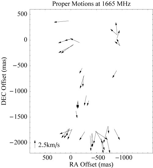
1665-MHz proper motions with a reference motion of (4, −1) km s −1 (RA, Dec.) added.

3.8 Statistical relationships
The large numbers of masers at 1665 MHz make it the best frequency for studying statistical relationships of properties of OH masers. The maser properties were tested for a variety of correlations, shown in Fig. 13.
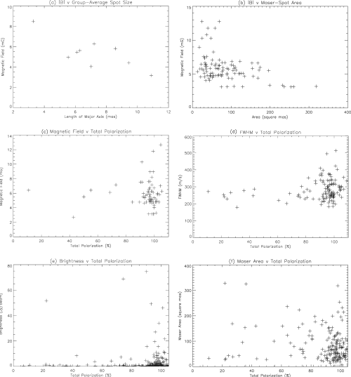
Charts showing likely relationships between various maser properties: (a) magnetic field strength versus group-averaged spot size; (b) magnetic field strength versus spot area; (c) magnetic field versus total polarization; (d) FWHM of feature spectrum versus total polarization; (e) maser brightness versus total polarization; (f) maser area versus total polarization.

There were no correlations found between maser FWHM and flux density, maser area, field strength or Dec. offset (position); 92 per cent of the masers for which FWHM was measured had widths between 200 and 400 m s −1. Note that there may be a selection effect at work at the lower end of the linewidth distribution; at least four channels were required for a Gaussian fit to be attempted. Extremely narrow lines therefore may not show emission in enough channels to allow a Gaussian fit, thus the sharp cut-off of masers with FWHM under 200 m s −1 should be regarded with caution. Neither maser area nor magnetic field strength was correlated with maser flux density. Most of the masers with area over 190 mas2 come from maser group d, which has already been noted for its extended masers; the rest come from the positional centre of group e.
There was no correlation found between maser area and total polarization, nor between maser flux density and total polarization, although the small number of low polarization masers makes this less clear. Three correlations were found, as follows.
FWHM with total polarization. Masers with total polarization below 80 per cent (and, typically, correspondingly low circular polarization values) tended to have below-average linewidths. No maser theories currently predict this.
Magnetic field strength with total polarization. There were no masers with high magnetic field strengths and low (<80 per cent) total polarizations. This is probably because the higher gas density presumed to accompany high magnetic field strengths enhances polarization through generally higher maser gain coefficients.
Magnetic field strength with maser area. Masers with high magnetic field strengths tend to be smaller. The work of Gray & Field (1994, 1995) has shown that maser amplification is enhanced along magnetic field lines, and that the maser beam angle is narrowed by this effect – a phenomenon they call ‘magnetic beaming’. Stronger magnetic fields could enhance this effect. The correlation is also probably related to the higher gas density presumed to accompany high magnetic field strengths; higher densities may allow higher amplification for a maser of any given size.
3.9 Two-point correlation
The large number of masers at 1665 MHz makes for a good two-point correlation, which is shown in Fig. 14.
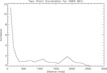
The two-point correlation of the 1665-MHz masers.

It has long been known that masers tend to cluster; Reid et al. (1980) suggested that the scale size in W3(OH) was 60 mas (∼120 au), but this work shows that in order to include faint outliers (which they did not detect) the maser clustering scale begins at about 300 mas (∼600 au) where the correlation function has fallen to 10 per cent of its initial value. The correlation shows a significant peak at just less than 2 arcsec (∼4000 au) in size. This is probably related to the size of the underlying UCH ii region. The size of this region depends on the observation frequency, being ∼1.5 arcsec at 15 GHz, but ∼3 arcsec at 1.6 GHz. Fig. 15 shows a zoom in on the first 300 mas of the correlation with smaller bins and higher resolution. It shows that the distribution within a maser cluster concentrates the masers ever more at closer distances, right down to between 10 and 20 mas (∼20 and ∼40 au). At around 8 mas, the correlation breaks down and suddenly drops to zero at 4 mas. This is because the beam size of the observation was about 8 mas, and so Gaussian fitting routines run into difficulties with masers which are less than 8 mas apart, and fail completely for masers less than 4 mas apart. The correlation function shows that masers cluster more strongly down to a scale that is comparable to their physical size. Our conclusions in this respect are therefore in accord with Reid et al. (1980), and the maser clustering clearly does not come from a fractal distribution, which would give a correlation function that is broadly scale-independent.
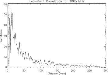
The two-point correlation of the 1665-MHz masers, restricted to separations of 300 mas or less, with smaller bins and hence ‘higher resolution’ than in Fig. 14.

4 Discussion and Conclusions
The data, at 1665 MHz, have given up a wealth of information. The positional distribution, velocity distribution and polarization information together paint a dynamic picture of the molecular environment around a UCH ii region. A complete catalogue of all maser emission with brightness above 75 mJy beam −1 is available at , and see also Wright (2001)
Study of the maser line shapes shows that deviations from Gaussian form are extremely rare. Minor deviations in the line wings (presumed to be from unsymmetrical rebroadening, but possibly also from blending with weak companions) are detected for a small proportion of the masers, but major deviations exist for just two cases, representing ∼1 per cent of the masers. One of these cases showed a true double peak and may be indicative of the only instance of negligible velocity redistribution conditions in the gas, because this is required for such ‘hole burning’. Future modelling of maser line shapes in star-forming regions will be constrained by the need to produce near-Gaussian form in the vast majority of cases. Predictions of peculiar multipeaked and multishouldered line shapes that have appeared in the literature were not borne out by the observations. The FWHM of the lines generally lay in the range of 200–400 m s −1, in agreement with Reid et al. (1980), although caution is required when interpreting the lower end of the range because a minimum of four channels was required for a fitting attempt. A statistical relationship was detected between the FWHM of a maser and the level of total polarization, whereby low levels of polarization were accompanied by narrow linewidths. As yet, no maser theories predict this relationship.
From the general splitting of the LCP and RCP emission, it is clear that the magnetic field generally points away from the observer (Garcia-Barretto et al. 1988). The polarization of the masers shows a clear trend: the further from the centre of the W3(OH) region the masers are, the more linear polarization and unpolarized emission they exhibit and the less circular and total polarization they contain. This is interpreted as indicating a general change in orientation of the ambient magnetic field, such that moving north or south of the centre results in an increase in the angle between the magnetic field axis and the line of sight. This description might indicate that the magnetic field lines point towards the central star, but we also discuss a disc interpretation below.
Interpreting coincident RCP and LCP maser components as Zeeman pairs not only clarifies the otherwise messy velocity distribution of the masers, but also gives valuable information about the magnetic field strengths. The magnetic field strength is found to be fairly constant within each maser cluster, with typical values of ∼5–7 mG. The exception is maser group c, which exhibits a wide range of magnetic field strengths from 5 to 13 mG. Relatively low field strengths are found in maser group d in the west of the region.
A correlation was found between the magnetic field strength and total polarization, where masers of high magnetic field strength always displayed high total polarization. A correlation was also found between the magnetic field strength and the size of the masers. This is an effect of ‘magnetic beaming’, which could be enhanced by stronger fields. Because stronger fields would also indicate higher densities, a maser cloud of smaller size can become strong enough to be detected.
Before ‘demagnetization’ the velocity distribution of the masers appears chaotic; after demagnetization, a clear pattern emerges: maser group c, which contains a large spread of magnetic field strengths, also contains a wide velocity dispersion and so appears much more chaotic. The masers in the far south-east are shown not to be part of this group, nor do they share the motion of the rest of the masers, but instead appear to be an outlying group. The rest (80 per cent) of the masers lie in a well-defined velocity trend from north to south. The evidence suggests a thick rotating disc or torus of minimum diameter 4600 au, aligned north–south around the central massive star – itself determined to have a lower mass limit of 8 M⊙. Using symmetry arguments for the dimensions of the disc, the stellar mass could be as high as 27 M⊙ and the disc diameter 7000 au. In a disc interpretation of W3(OH) it is unlikely that the magnetic field lines in the disc lie radially, because the differential rotation in a disc would quickly wind the field lines up into a tight spiral. What is more likely is that with a 10° inclination of the disc we are seeing the field entering the disc from ‘above’ or ‘below’.
The special nature of maser group c was noted in reference to observations of OH excited states and methanol lines, which are both strong in this area. The phenomenon that is powering this cluster of masers sustains many lines and leads to a wide velocity spread. Also, as shown by magnetic field measurements, this group contains denser clumps of gas than the rest of the region.
The proper motion of the masers measured between 1978 and 1997 agrees very well with the measurement of Bloemhof et al. (1992) between 1978 and 1986. In the light of the rotational motion suggested by the velocity gradient, a different model is proposed to that proposed by Bloemhof et al. The proper motions are consistent with a north–south rotating disc of material at an angle of inclination to the line of sight of 10°, with the exception of the group of northern masers already noted as exceptional. A value is adopted for the unknown proper motion of the reference maser that both emphasizes the rotation of the disc and also places the exceptional maser group in motion away from the disc in an orthogonal direction – indicative of motion in an outflow. The present work reproduces the generally divergent motion of the masers, so the motions in the source must include an element of expansion in addition to rotation. Such an element of divergence within the disc could indicate that we are witnessing its destruction.
The two-point correlation on such a large sample of masers has produced a larger clustering scale than found by Reid et al. (1980), whose observations estimated the cluster size at ∼60 mas (120 au), but it is shown that inclusion of all faint outliers increases the clustering scale to ∼300 mas (600 au). However, the increase in clustering scale is a result of the better sensitivity of the present observations, and is not in conflict with the conclusions of Reid et al. The density of masers increases at smaller scalelengths until the correlation breaks down at the resolution limit.
Acknowledgments
MMW thanks the Engineering and Physical Sciences Research Council (EPSRC) for funding him as a postgraduate student. We would like to thank the referee, Professor Mark Reid, for his comments that have helped us to improve this paper and Paper II. The NRAO is a facility of the National Science Foundation operated under cooperative agreement by Associated Universities, Inc.
References